
CHAPTER 16
Regime Shifts
THE CHALLENGE
Investors want to grow wealth and avoid large drawdowns along the way. But portfolios with higher expected returns also carry greater risk. Faced with this trade‐off, investors choose portfolios that optimally balance their goal to grow wealth with their aversion to risk. This approach to portfolio selection implicitly assumes that risk is stable through time, which is far from true.
In Chapter 13, we showed that accounting for stability in portfolio construction helps to stabilize portfolio risk by reducing a portfolio's dependence on asset classes with unstable risk profiles. But even stability‐adjusted portfolios experience large swings in standard deviations through time. As an alternative, we could engineer a portfolio to perform well in a given regime, with the hope that it holds its own when that regime does not come to pass. This strategy, like stability‐adjusted optimization, selects a set of fixed weights, but it is constructed to perform well in a particular regime that we fear the most or which we believe is most likely to occur. Unfortunately, this approach is also subject to large swings in portfolio risk. It is hard to stabilize the risk of a portfolio that has fixed weights.
It may be preferable to allow our portfolio's asset mix to change through time. If we successfully predict future investment conditions, we should be able to outperform a static asset mix with tactical tilts. Of course, if our predictions are wrong, tactical trading may harm the portfolio more than it helps it. Furthermore, tactical strategies must add enough value to overcome the incremental trading costs they incur. This begs the question: Are markets sufficiently macroinefficient to justify tactical asset allocation, or is this pursuit merely a fool's errand?
PREDICTABILITY OF RETURN AND RISK
Let's begin by distinguishing between the predictability of return and the predictability of risk. Predicting returns successfully is more valuable than predicting risk successfully, but it is also more difficult. According to the efficient markets hypothesis, asset returns follow a random walk. Assets cannot stray far from their fair value, the story goes, because arbitrageurs quickly buy undervalued assets and sell overvalued assets in pursuit of profits. Although this logic may only apply in a limited sense to small or illiquid markets where assets are expensive to trade, it should hold reasonably well for asset classes such as large‐capitalization stocks and government bonds. Yet even in highly liquid markets, some—notably Paul A. Samuelson—have argued that markets are macroinefficient because arbitrageurs lack sufficient capital, or risk appetite, to correct widespread mispricing across aggregations of thousands of securities the way they do for individual securities. Therefore, skilled investors might be able to predict asset class returns with some degree of reliability, though this is still a very challenging task.
Predicting risk is easier. The economic forces that affect long‐run returns might not apply to the volatility of returns. Volatility—which we measure as the standard deviation of returns—arises from uncertainty about an asset's true value. In short, prices fluctuate when new information becomes available and investors react to it. Volatility depends on the significance of new information and the pace at which it arrives, and there are no fundamental laws governing how these processes should unfold. In other words, volatility lacks a clear equilibrium value. In fact, it is often the case that volatility clusters into regimes of high volatility and regimes of low volatility, which means it is partly predictable. This fact does not contradict the notion of an efficient market.
In this chapter, we investigate the use of regimes to manage risk, not to predict the direction of returns. We present two approaches for dealing with regime shifts. The first is regime‐sensitive asset allocation, and the second is tactical asset allocation.
REGIME‐SENSITIVE ALLOCATION
Figure 16.1 shows the monthly correlation between U.S. equities and Treasury bonds for nonoverlapping five‐year periods as one example of the variability of risk. The gains and losses experienced by stocks and bonds generally aligned during the 1980s and 1990s, possibly due to their common sensitivity to interest rates and inflation. After that, their correlation turned sharply negative. Stocks and bonds became polarized as risky and safe, respectively, and they moved in opposite directions most of the time.

FIGURE 16.1 Monthly Correlation of U.S. Equities and Treasury Bonds (Five‐Year Rolling Subsamples)
Given the variability in the correlation of stocks and bonds, we might choose to define regimes based on macroeconomic variables such as inflation or interest rate policy. Alternatively, we could define regimes directly from the correlation between stocks and bonds. Both of these approaches are reasonable, but they consider the performance only of stocks and bonds. It might be better to define regimes in a way that captures the behavior of our entire investment universe. One way to do this is with a multivariate measure of financial turbulence.
Financial Turbulence
In Chapter 12, we introduced financial turbulence, which is based on a statistical quantity called the Mahalanobis distance.1 In a single number, financial turbulence characterizes the degree of unusualness in a cross section of asset class returns. It captures not only extreme price moves but also unusual correlations that affect a portfolio's diversification. The turbulence score for any given month ![]() , equals:
, equals:
In Equation (16.1), ![]() is a vector of monthly returns across asset classes,
is a vector of monthly returns across asset classes, ![]() is a vector of average returns for each asset class over the full 40‐year sample, and
is a vector of average returns for each asset class over the full 40‐year sample, and ![]() is the inverse of the covariance matrix computed from the 40‐year sample. We multiply by
is the inverse of the covariance matrix computed from the 40‐year sample. We multiply by ![]() so that the expected value of turbulence equals 1. The inverse covariance matrix puts the monthly returns in context, and this step is critically important. For example, stock prices may regularly move by 5 or 10 percent per month, but for bonds these returns would be extreme. Likewise, the divergence of two asset classes is surprising if they are positively correlated, but not if they are negatively correlated. The inverse covariance matrix embeds all of the expected relationships across asset classes, based on the full sample of data.
so that the expected value of turbulence equals 1. The inverse covariance matrix puts the monthly returns in context, and this step is critically important. For example, stock prices may regularly move by 5 or 10 percent per month, but for bonds these returns would be extreme. Likewise, the divergence of two asset classes is surprising if they are positively correlated, but not if they are negatively correlated. The inverse covariance matrix embeds all of the expected relationships across asset classes, based on the full sample of data.
We apply this formula to the six major asset classes in our empirical example (excluding cash equivalents): U.S. equities, foreign developed market equities, emerging market equities, Treasury bonds, corporate bonds, and commodities. Figure 16.2 shows historical monthly turbulence since 1976. It clearly spikes during well‐known events such as the Black Monday stock market crash of 1987, the Russian debt default in 1998, and the global financial crisis in 2008. It also flags some less obvious periods of stress. These events carry important consequences for portfolio risk, even if they do not make newspaper headlines.

FIGURE 16.2 Financial Turbulence
Portfolio Construction with Conditional Risk Estimates
Regime variables are informative if they describe differences in investment performance. Financial turbulence passes this test. Table 16.1 shows asset class standard deviations and correlations corresponding to the 10 percent most turbulent months, which we call the turbulent sample, and the remaining 90 percent of months, which we call the nonturbulent sample.
TABLE 16.1 Risk Characteristics in Turbulent and Nonturbulent Regimes
| Correlations | ||||||
| Standard | U.S. | Foreign | EM | Treasury | Corporate | |
| Deviations | Equities | Equities | Equities | Bonds | Bonds | |
| Turbulent | ||||||
| U.S. Equities | 27.4% | |||||
| Foreign Developed Market Equities | 29.6% | 0.74 | ||||
| Emerging Market Equities | 33.5% | 0.86 | 0.76 | |||
| Treasury Bonds | 11.7% | 0.22 | 0.16 | 0.25 | ||
| U.S. Corporate Bonds | 16.3% | 0.44 | 0.39 | 0.49 | 0.84 | |
| Commodities | 27.6% | 0.29 | 0.27 | 0.31 | −0.10 | 0.09 |
| Nonturbulent | ||||||
| U.S. Equities | 14.0% | |||||
| Foreign Developed Market Equities | 15.9% | 0.60 | ||||
| Emerging Market Equities | 23.6% | 0.51 | 0.61 | |||
| Treasury Bonds | 4.7% | 0.06 | −0.01 | −0.09 | ||
| U.S. Corporate Bonds | 5.6% | 0.23 | 0.15 | 0.11 | 0.89 | |
| Commodities | 19.1% | 0.10 | 0.28 | 0.25 | −0.04 | −0.01 |
| Difference | ||||||
| U.S. Equities | 13.4% | |||||
| Foreign Developed Market Equities | 13.7% | 0.14 | ||||
| Emerging Market Equities | 9.9% | 0.34 | 0.15 | |||
| Treasury Bonds | 7.0% | 0.16 | 0.17 | 0.33 | ||
| U.S. Corporate Bonds | 10.7% | 0.20 | 0.24 | 0.38 | −0.05 | |
| Commodities | 8.5% | 0.19 | −0.02 | 0.06 | −0.05 | 0.10 |
Standard deviations are much higher during turbulent periods, as we should expect. Most of the correlations also increase when conditions are turbulent; hence, there is less potential for diversification. These conditions usually cause traditional portfolios to perform poorly. Should we optimize our portfolio for turbulent regimes instead? We can, but we face the following trade‐off. The more we engineer a portfolio to protect it from financial turbulence, the more we sacrifice optimality in nonturbulent periods. On the other hand, if we choose a portfolio that is optimized for nonturbulent times, we should brace for discomfort when turbulence occurs. Perhaps we should compromise, by tilting our portfolio toward asset classes that are more resilient to turbulence. Ideally, the portfolio will perform well when turbulence prevails without underperforming significantly during nonturbulent periods.
To implement this strategy, we optimize a portfolio based on a covariance matrix that blends covariances from both regimes. In our example, we use a simple average of the turbulent and nonturbulent covariance matrices. Because the turbulent sample represents only 10 percent of history, a 50 percent weight constitutes a substantial tilt toward the estimates that prevailed during turbulent regimes. Table 16.2 shows the moderate portfolio from Chapter 2 alongside a new portfolio based on the turbulence‐conditioned covariance matrix. The allocations are meaningfully different, even though both portfolios target a 7.5 percent return and use the same expected return assumptions. The blended‐covariance solution favors emerging market equities compared to U.S. equities, and it substitutes cash equivalents for corporate bonds. The full‐sample standard deviation increases from 10.8 percent to 11.5 percent, and the standard deviation in nonturbulent periods increases from 8.8 percent to 9.8 percent. However, the new portfolio reduces the standard deviation during turbulent regimes from 18.8 percent to 17.0 percent. This trade‐off may or may not be worthwhile. The benefit this portfolio provides in turbulent regimes is modest. Moreover, we receive this benefit only 10 percent of the time, while we experience the cost of higher volatility 90 percent of the time. This result underscores the limitation of a static asset mix.
TABLE 16.2 Full‐Sample and Regime‐Conditioned Optimal Portfolios
| Full‐Sample | Blended | |
| Optimal Allocations | Covariances | Covariances |
| U.S. Equities | 25.5% | 8.6% |
| Foreign Developed Market Equities | 23.2% | 21.0% |
| Emerging Market Equities | 9.1% | 26.0% |
| Treasury Bonds | 14.3% | 9.9% |
| U.S. Corporate Bonds | 22.0% | 0.0% |
| Commodities | 5.9% | 6.4% |
| Cash Equivalents | 0.0% | 28.1% |
| Expected Return | 7.5% | 7.5% |
| Full‐Sample Standard Deviation | 10.8% | 11.5% |
| Nonturbulent Regime Standard Deviation | 8.8% | 9.8% |
| Turbulent Regime Standard Deviation | 18.8% | 17.0% |
TACTICAL ASSET ALLOCATION
In contrast to portfolio rebalancing, which serves merely to restore the portfolio's optimal weights when price changes cause the asset class weights to drift away from their optimal targets, tactical asset allocation shifts a portfolio's composition proactively in response to some signal. To succeed, tactical asset allocation should add more value when it is correct than it subtracts when it is wrong. Or it should be correct sufficiently often to compensate for its losses, on average. Overall, it must enhance expected utility compared to the static alternative, net of costs. To do this we need a predictive signal and a way to translate that signal into an investment decision.
Identifying a Predictive Signal
A good predictive signal is necessary, but not sufficient, to create a profitable tactical asset allocation strategy. Some investors might prefer to rely on their qualitative judgment, but we focus here on data‐driven signals, in part because they are naturally more transparent and replicable. Let's continue with our analysis of turbulence. As we soon show, turbulence is predictive by virtue of its persistence.
There are, of course, other signals that might add value. Economic indicators such as growth and inflation might be valuable. Another indicator that has gained widespread traction in recent years is the absorption ratio, introduced by Kritzman, Li, Page, and Rigobon (2011). Like turbulence, it is derived statistically and based on asset prices. Whereas turbulence represents extreme dislocations in asset prices, the absorption ratio reveals whether the risk within an asset universe is highly concentrated or diffuse. When a small set of factors explains a large fraction of total risk, portfolios composed from those assets are vulnerable to large drawdowns because shocks tend to propagate quickly and broadly in such a setting. When risk is broadly distributed across many factors, negative shocks are more likely to have a localized and contained effect on portfolios. The absorption ratio is based on Principal Components Analysis (described in detail in Chapter 18). It equals the fraction of total variation in returns that is explained—or absorbed—by a subset of the most important statistical factors. Statistical factors are nothing more than sets of portfolio weights across a universe of assets, chosen in such a way that they are all uncorrelated and explain successively smaller fractions of total risk. Statistical factors do not have descriptive names, but they are convenient in that they always explain variation in the data as efficiently as possible.
We do not include empirical tests of economic indicators or the absorption ratio here, but the technique we are about to describe using financial turbulence applies as well to economic variables and the absorption ratio.
Detecting Regimes: Hidden Markov Models
We begin by defining a regime as a period in which an indicator, in this case financial turbulence, is above or below a particular threshold. We might devise a trading rule that positions a portfolio more defensively when turbulence is elevated and more aggressively when it is not. Even a simple rule like this might add value. However, simple thresholds have three important limitations. First, they fail to recognize persistence, which can lead to excessive trading. Second, by focusing only on the level of the indicator, this rule fails to account for shifts in its volatility, which may offer additional insight. Third, such a rule is sensitive to the choice of the threshold, which in many cases is an arbitrary choice.
Hidden Markov models offer a more sophisticated alternative. These models presume that the data we observe emanates from multiple regimes, each of which has a degree of persistence from one period to the next. For example, if we are in regime A this month, regime A might be more likely to prevail next month as well. But there is also a chance that the regime will shift abruptly from A to B. The term “Markov” refers to the assumption that the underlying regime variable follows a Markov process in that next period's regime probability depends only on the regime we are in today. Unfortunately, we never know for certain which regime we are in, even with the benefit of hindsight. As their name suggests, the regimes in hidden Markov models are indeed hidden variables (sometimes called latent variables). We rely on a statistical method called Maximum Likelihood Estimation (MLE) to infer from the data which regime is most likely to explain each observation, given all the data that preceded and followed it. The solution is obtained by using a well‐known and highly reliable search method called the Baum‐Welch algorithm. (See the Appendix to this chapter for more detail.) By allowing for the presence of multiple regimes, we are better able to explain the complex behavior of many real‐world variables. Recall from Chapter 13 that the composite mixture of two normal distributions does not yield another normal distribution, but a fat‐tailed one.
Kritzman, Page, and Turkington (2012) use hidden Markov models to solve for the two normal distributions and regime transition probabilities that best explain historical data for U.S. gross national product, U.S. consumer price index, and market turbulence in U.S. equities and currencies. In an intentionally contrived example in which data is drawn from known regimes that switch over time, the authors show that the true underlying behavior is much more likely to be recovered by a hidden Markov model than a simple threshold. They also provide empirical evidence that economic data conforms to regimes. The authors demonstrate that relatively simple regime‐switching strategies across risk premiums and asset classes outperform their static investment alternatives.
Let's explore a case study to make these concepts more tangible. We use financial turbulence as our regime indicator. The only parameters we need to specify are the number of regimes and the type of distribution we envision for our variable of interest in each regime. The model determines everything else. For this example, we ask the model to identify three distinct regimes that best explain historical turbulence.2 It returns to us a transition matrix stating the probability of occurrence for each regime in the next period as a condition of the regime that prevails in the current period. The top panel of Table 16.3 shows the results of the model. We see that regime persistence, which comes from the diagonal entries of the transition matrix, is above 50 percent in all cases, which indicates predictive potential. We also see that it varies across regimes. The first regime, which happens to be the most persistent, has low average turbulence and low dispersion in outcomes. We label it “calm.” We label the second regime “moderate” because it is characterized by a higher average return and a higher standard deviation. Finally, the third regime represents “turbulent” conditions. It is the least stable, yet still predictive. Keep in mind that we do not predetermine how the persistence, averages, and standard deviations align across regimes. The fact that regimes with worse investment conditions on average are also more uncertain and more fleeting is a feature of markets that turbulence and the hidden Markov model have jointly uncovered. If we tried to fit the same model on random data, it would either fail to find a solution or it would produce three indistinguishable regimes.
TABLE 16.3 Hidden Markov Model Fit and Conditional Asset Class Performance
| Calm | Moderate | Turbulent | |
| Regime Persistence | 92% | 75% | 67% |
| Turbulence Average | 0.7 | 1.1 | 1.7 |
| Turbulence Standard Deviation | 0.2 | 0.3 | 0.6 |
| Average Annual Return | |||
| U.S. Equities | 15.0% | 13.6% | −27.7% |
| Foreign Developed Market Equities | 15.3% | 5.7% | −12.0% |
| Emerging Market Equities | 17.2% | 21.7% | −26.0% |
| Treasury Bonds | 5.9% | 9.6% | 12.3% |
| U.S. Corporate Bonds | 7.5% | 10.2% | 4.2% |
| Commodities | 7.8% | 7.8% | −17.1% |
| Cash Equivalents | 3.9% | 5.9% | 7.4% |
| Standard Deviation | |||
| U.S. Equities | 12.6% | 20.2% | 19.9% |
| Foreign Developed Market Equities | 14.7% | 19.6% | 31.0% |
| Emerging Market Equities | 21.3% | 30.5% | 32.5% |
| Treasury Bonds | 4.2% | 6.4% | 12.1% |
| U.S. Corporate Bonds | 5.1% | 7.8% | 16.6% |
| Commodities | 18.1% | 21.3% | 30.3% |
| Cash Equivalents | 0.8% | 1.1% | 1.7% |
Now that we know more about the dynamics of turbulence, we link this information to asset class returns. The middle panel of Table 16.3 shows the average annualized return of our seven asset classes in each regime, and the bottom panel presents standard deviations. Again, recall that even with hindsight we do not know for certain which regime corresponds to each month in history. For this analysis, we simply assign the most likely regime to each month. Our findings are intuitive: Calm periods are kind to investments, moderate periods have markedly elevated volatility despite sometimes‐higher mean returns, and turbulent periods have very high risk and typically negative average returns. Figure 16.3 shows the probabilities associated with each regime through time.

FIGURE 16.3 Hidden Markov Model Regime Probabilities
Testing out of Sample
To test the efficacy of our tactical asset allocation rule, we perform an out‐of‐sample backtest in which tactical decisions rely only on data available at each point in time. Our original turbulence calculation uses information spanning the entire 40‐year sample, so we must recalculate it. Each month, we compute turbulence using the formula shown previously, but now we estimate means and covariances using the prior 60 months of returns. This process produces turbulence data starting in 1980. Next, we calibrate the hidden Markov model using historical data only. Starting in December 1990, we calibrate the model using the prior 10 years of turbulence, and we append new data each month to form a growing lookback window on which we recalibrate the model. Figure 16.4 shows the probability forecast of each regime per month, out of sample. Each month, the model supplies an updated probability that the current regime is calm, moderate, or turbulent. Next, we forecast the probability that each regime will prevail next month by using the transition matrix to project the current regime probabilities forward one period. For example, the probability that regime A will prevail next month is equal to the probability that we are currently in regime A times the probability of remaining in regime A, plus the probability that we are currently in regime B times the probability of transitioning from B to A, plus the probability that we are currently in regime C times the probability of transitioning from C to A. The next‐period probability of each regime, ![]() , is described succinctly by the product of the transition matrix of conditional regime probabilities and the current regime probabilities,
, is described succinctly by the product of the transition matrix of conditional regime probabilities and the current regime probabilities, ![]() :
:

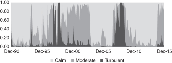
FIGURE 16.4 Hidden Markov Model Regime Probability Forecasts (Out of Sample)
Figure 16.4 shows the probability forecast of each forthcoming regime per month, out of sample.
There are many ways to specify portfolio weights using the regime signals in Figure 16.4. For illustration, we use the conservative, moderate, and aggressive portfolios from Chapter 2 and blend them in proportion to the regime probabilities at the end of each month. We then record the returns of each portfolio as well as the tactically blended portfolio over the following month. This rule depends on very few parameters, and it smoothly transitions the portfolio's composition among a conservative, moderate, and aggressive asset mix as regime probabilities shift. Table 16.4 and Figure 16.5 show that the tactical strategy produced the largest cumulative return, with a standard deviation substantially below that of the aggressive portfolio. It delivered a higher Sharpe ratio than the conservative portfolio at a return level 2.6 percent higher. We have little doubt that we could produce performance that is more compelling by devising more sophisticated strategies involving additional indicators, conditional return forecasts, and reoptimized conditional allocations. Also, though we have not adjusted our results for transaction costs, the amount of trading involved here is certainly reasonable and can be dialed up or down using trading thresholds, minimum holding periods, and other techniques.
TABLE 16.4 Backtest Performance
| Conservative | Moderate | Aggressive | Tactical | |
| Annual Return | 6.0% | 7.6% | 8.1% | 8.6% |
| Annual Standard Deviation | 6.0% | 9.6% | 13.8% | 10.3% |
| Sharpe Ratio | 0.54 | 0.50 | 0.38 | 0.57 |
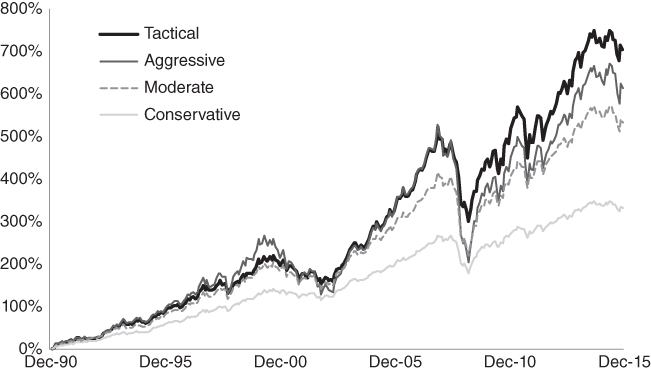
FIGURE 16.5 Cumulative Returns
THE BOTTOM LINE
The fact that risk varies through time presents a challenge, but also an opportunity. We have proposed three methods for stabilizing portfolio risk. The first is stability‐adjusted optimization, which we discussed in Chapter 13. It identifies portfolios that are less dependent on asset classes with relatively unstable risk profiles. The second method is to define a particular regime and to optimize for a portfolio that is more sensitive to the covariances that prevailed during that regime. Ideally, this regime‐sensitive portfolio will perform well when the regime occurs, while holding its own the rest of the time. Both of these approaches yield static portfolios that most likely will still experience wide swings in their volatility. The third method is to shift a portfolio's asset mix tactically based on regime indicators. By allowing weights to change in response to market conditions, tactical strategies are less constrained; therefore, they present greater flexibility than static portfolios. Although this additional flexibility may not always improve performance, we have provided encouraging evidence to suggest that some investors might profit from tactical trading, given the right insights and methods.
APPENDIX: BAUM‐WELCH ALGORITHM
To fit a hidden Markov model to data, we select a characteristic to distinguish regimes, and we find the probability of transitioning from one regime to another, given our sample of historical values for the regime characteristic. Thankfully, the Baum‐Welch algorithm turns this potentially laborious search into a computationally straightforward exercise. Its effectiveness stems from the use of both forward and backward search procedures, from which information is combined, refined, and recycled iteratively to get better and better estimates. A thorough discussion of the algorithm is beyond the scope of this book, but it is documented in detail by Baum, Petrle, Soules, and Weiss (1970) and others. Kritzman, Page, and Turkington (2012) offer an intuitive description with a simple example. Interested readers should refer to these other sources for mathematical details, but we provide some intuition below.
We implement the Baum‐Welch algorithm by first guessing the probabilities of shifting from one regime to another, along with the mean and standard deviation of the regime characteristic for each regime. (In our case study, we used turbulence as the regime‐defining characteristic.) These initial guesses are chosen arbitrarily. The algorithm then computes what are called “forward probabilities.” For the first period, the algorithm evaluates the likelihood of each regime based on our initial guesses, together with that period's value for the regime characteristic and the distribution of the characteristic for each regime. For the next period, the algorithm evaluates the likelihood of each regime based on the new value of the characteristic and the same initial guesses, and accounting for the likelihood of each regime from the prior period. It iterates forward in this fashion until we have forward probabilities for every time period. We now have a time series for each regime that tells us how likely it is that we would observe that value for the regime characteristic given the distribution of the characteristic for each regime, based on everything that occurred previously. The algorithm captures the fact that some values for the regime characteristic are more likely to have come from one regime than another, given their distributions. It also captures the fact that a regime is more likely if it is highly persistent and believed to have prevailed in the preceding months.
Next, the algorithm follows the same procedure in reverse, to generate backward probabilities. It then combines the forward probabilities and backward probabilities into “smoothed probabilities.” In essence, these smoothed probabilities tell us the likelihood of each regime at each point in time, given what regimes were likely to have occurred before and after.
To summarize, the Baum‐Welch algorithm applies forward and backward iteration to an initial set of assumptions to determine the relative likelihood of each regime at each point in time. The next step is the critical component that allows this algorithm to work. The algorithm uses the regime probabilities to form a new and better set of estimates for all of the parameters. For example, it calculates the probability that each pair of successive observations of the regime characteristic comes from regime A “transitioning” to stay in regime A, divided by the probability of regime A overall. This produces a new and improved estimate of the first element in the transition matrix. Likewise, using information about which periods are most likely to be in regime A, the algorithm estimates the mean and standard deviation of the characteristic's distribution for regime A. These estimates also improve the original guesses. We then enter these new estimates into the algorithm and repeat the entire process. The estimates continually improve after each iteration, and they ultimately converge to a stable solution that best describes regime behavior in our sample of characteristic values. Technically speaking, the algorithm is only guaranteed to converge to a “local solution,” but, based on our experience we find that it converges to stable and plausible parameters consistently.
REFERENCES
- L. Baum, T. Petrle, G. Soules, and N. Weiss. 1970. “A Maximization Technique Occurring in the Statistical Analysis of Probabilistic Functions of Markov Chains,” Annals of Mathematical Statistics, Vol. 41, No. 1.
- G. Chow, E. Jacquier, M. Kritzman, and K. Lowry. 1999. “Optimal Portfolios in Good Times and Bad,” Financial Analysts Journal, Vol. 55, No. 3 (May/June).
- M. Kritzman, K. Lowry, and A‐S. Van Royen. 2001. “Risk, Regimes, and Overconfidence,” Journal of Derivatives, Vol. 8, No. 3 (Spring).
- M. Kritzman, S. Page, and D. Turkington. 2012. “Regime Shifts: Implications for Dynamic Strategies,” Financial Analysts Journal, Vol. 68, No. 3 (May/June).
- M. Kritzman, Y. Li, S. Page, and R. Rigobon. 2011. “Principal Components as a Measure of Systemic Risk,” Journal of Portfolio Management, Vol. 37, No. 4 (Summer).
- M. Kritzman and Y. Li. 2010. “Skulls, Financial Turbulence and Risk Management,” Financial Analysts Journal, Vol. 66, No. 5 (September/October).