Overview
In this chapter, we intend to foray into matrices and their applications using Python. We will look at different matrix manipulation techniques that will help us use them efficiently to build useful tools in real-world applications.
By the end of this chapter, you will understand matrices and be able to perform operations on them. You will implement one of the applications of matrices, known as Markov chains, using transition matrices and then use Markov chains and the Markov property to solve real-world problems.
Introduction
A matrix is a rectangular array of numbers or expressions arranged in rows and columns and considered as a single entity. As we are considering a matrix as a single object, if we perform an operation on it, it will apply to each of the elements within it:

Figure 6.1: A simple m × n matrix with m rows and n columns
A simple linear single-dimension array rarely suffices for the physical world we live in, and almost all attributes related to space and time require more than one dimension. Compactness is one of the main reasons for the use of matrices. A matrix is compact when it is closed and bounded or simply has its points within a fixed distance of one another. Primarily for these two reasons, matrices find applications in practically every field, including fundamental mathematical concepts, ranging from graph theory, linear transformations, and probability theory, to different branches of physics, such as quantum mechanics and electromagnetism.
The Markov chain model and its variations are one such application, tying concepts of matrices, limits, and probability together to produce results in real-world problems where uncertainty is predominant. In a mathematical space, whenever there is uncertainty, decisions are based on probability; this forms the basis of Markov chains. These use a specific type of matrix, called a transition matrix, to build state diagrams. A Markov chain is effectively a memoryless process that is primarily based on the current state to decide the outcome of the next state. We find their application in some very important use cases, including page-rank algorithms, autocomplete applications, and text generators. We will be studying these concepts in more detail later in the chapter, and for that, we need to first understand matrices.
Matrix Operations on a Single Matrix
In this chapter, we will study the different ways of manipulating matrices and how to implement them in Python. Understanding how a matrix works broadly means understanding the fundamentals of how 2D or multidimensional arrays work. Once we have a good understanding of the basics of 2D matrices, those interested can delve into advanced studies of matrices, which includes special types of matrices such as sparse matrices, vector spaces, eigenvalues, and eigenvectors, which can involve more than two dimensions.
Matrices in Python can be implemented using either lists or arrays. Nested lists in Python work perfectly fine, but Python has a powerful package that makes matrix implementation much easier called NumPy. SciPy is another package that helps in matrix manipulation, but it is usually more suitable for larger matrix computations. We will be using both of these modules throughout this chapter.
Basic Operations on a Matrix
It is assumed at this point that you have the Python and its default libraries installed for running a basic Python program.
Once you have the package in place, let's define our first matrix:
# Importing Numpy package
import numpy as np
# Initializing and printing matrix z
x = np.array([[1, 2], [3, 4]])
print(x)
This matrix is the same as the following matrix, z, which is simply better represented and, as a good practice, is advisable whenever possible:
# Initializing and printing matrix z
z = np.array([[1, 2],
[3, 4]])
print(type(z))
Note that in the preceding code, we have printed the type of the variable z. Can you guess the output? The output should be as follows:
<type 'numpy.ndarray'>
The ndarray is the standard array format used by NumPy. The array object is homogenous, multidimensional, and has a data type object that is associated with it internally depending on its assignment.
For example, let's take an element in matrix z, which we defined previously:
# Printing the data types for matrix-z
print(z)
print(type(z))
print(z[0][1])
print(type(z[0][1]))
This produces the following output:
[[1 2]
[3 4]]
[[5 6]
[7 8]]
<type 'numpy.ndarray'>
2
<type 'numpy.int64'>
[Finished in 0.221s]
We find that the elements of the given matrix are of the int64 type, that is, the 64-bit integer type. Other data types include np.float32, np.complex, np.bool, np.object, np.string_, and np.unicode_.
For now, it is enough to know that pretty much every data structure that we build uses Python version 3.8 and NumPy version 1.17. As of the date of publication, NumPy has a special class called a matrix class that does pretty much the same things that ndarray does. The only difference is that the matrix class maintains its 2D nature and has some operators built in, such as * for multiplication and ** for power. Although the matrix class might come in handy and can be explored, the official NumPy documentation advises using a regular ndarray instead of np.matrix as it may be removed in the future. So, it is good to note here that the term ndarray in this context can be considered synonymous with the term matrix and will be used interchangeably in this chapter.
Let's continue working with ndarray. Assuming we have a single matrix, we will see some of the simple operations that we can do with it. We can use the same matrix, z, that we defined previously.
Let's print the sum of the elements:
# Sum of all elements of the matrix
print(z)
print(np.sum(z))
This produces the following output:
[[1 2]
[3 4]]
10
[Finished in 0.237s]
This is pretty straightforward. Let's now look at some other things that we can do.
Let's find the maximum, minimum, mean, and standard deviation of the z matrix:
# Value of the largest integer in the matrix
print("Max ", np.max(z))
# Value of the smallest integer in the matrix
print("Min ", np.min(z))
# Mean of elements in the matrix
print("Mean ", np.mean(z))
# Standard deviation
print("Standard deviation ", np.std(z))
This produces the following output:
('Max ', 4)
('Min ', 1)
('Mean ', 2.5)
('Standard deviation ', 1.1180339887498949)
[Finished in 0.207s]
There are a number of other operations that can be performed on an ndarray, including common mathematical functions such as sin, cos, log, and square root, and statistical functions, such as finding correlation coefficients and the cumulative sum, some of which we will be using shortly.
Inspecting a Matrix
Now, we will deal with some useful functions that can help us learn more about any array that we are working with. Let's continue to use the same matrix/ndarray, z, that we have been using so far:
- Let's print the information of a matrix:
# 1. Information about a matrix
print("Information: ")
print(np.info(z))
The output will be as follows:
Information:
class: ndarray
shape: (2, 2)
strides: (16, 8)
itemsize: 8
aligned: True
contiguous: True
fortran: False
data pointer: 0x7ff57665fef0
byteorder: little
byteswap: False
type: int64
None
- Now, to ascertain the shape of the matrix, write the following code:
# 2. Gives the shape of the matrix
print("Shape: ")
print(np.shape(z))
The output will be as follows:
Shape:
(2, 2)
- To check whether the matrix is a 2D or 3D matrix, write the following code:
# 3. Dimensions of the matrix
print("Dimensions: ")
print(np.ndim(z))
The output will be as follows:
Dimensions:
2
- To print the data type of the matrix, use the following code:
# 4. Data type of the matrix
print("Data type of elements")
print(z.dtype.name)
The output will be as follows:
Data type of elements
int64
- To print the length of the matrix, use the following code:
print("Length of the ndarray: ")
print(len(z))
The output will be as follows:
Length of the ndarray:
2
As we can see, the info function already displays the values of the other two functions we have called, namely, shape and type. Nevertheless, these functions serve a limited purpose, and that is all that is required sometimes. The multidimensional ndarray, as we know, is an array of arrays, and the len function of the NumPy array will always be the length of the first dimension. If z is a 2D matrix, then len(z) will be the number of rows in z.
In the following exercise, we will create a matrix. We can pretty much create a matrix with a nested list, but this problem will elaborate on how matrices are packaged and utilized in the real world.
Exercise 6.01: Calculating the Time Taken for Sunlight to Reach Earth Each Day
In this exercise, we will calculate the time it takes for sunlight to reach the Earth each day of the year.
As we know, the Earth revolves around the Sun in an elliptical orbit. As such, the distance between the Earth and the Sun changes, which will change the amount of time it takes for light to reach the Earth. There are three main equations that we can use to deal with this.
The mathematical formula to calculate time is as follows:

Figure 6.2: Formula to calculate time
We need to calculate the distance, r, between the Earth and the Sun:

Figure 6.3: Formula to calculate distance
In the preceding equation, the value of a is 149,600,000 km, which is the semi-major axis distance, e is 0.0167, which is the eccentricity of Earth's orbit, and θ is the angle from perihelion.
The dependent variable θ that will be required in the preceding equation is calculated as follows:

Figure 6.4: Formula for calculating the dependent variable
Note here that n is the number of days from the perihelion that occurs on January 3rd. To keep things simple, we will take this to be the beginning of the year.
Do not get bogged down by these equations as they are nothing but simple mathematical multiplications of constants and can be easily solved by a nifty Python library called math.
Let's now get started with the exercise:
- First, import the math and numpy libraries:
import math
import numpy as np
We will be using these libraries later.
- Next, define the two constants and use capitalization, which is the standard Python practice for naming these constants:
def earth_sun_distance():
# Semi-major axis between earth and sun
A = 149600000
# Eccentricity of earth
E = 0.0167
l = []
A here is the semi-major axis distance between the Earth and the Sun.
E is known as the eccentricity of the Earth.
l is a list that we have initialized for storing the values later.
- Let's jump into the main part of the code. For each of the 365 days, calculate theta, as it is different for each day of the year. Then, calculate the distance of the Earth from the Sun, and finally append that distance to a list:
# Calculating the distance between earth and sun
for i in range(365):
theta = (2 * math.pi * i) / 365.25
r = A*(1 - E**2) / (1 - (E * math.cos(theta)))
l.append(r)
return l
Note the use of the math.pi and math.cos functions from the math library that we imported previously.
- Calculate the time required in seconds, assuming the speed of light to be a constant value of 299,792 km/s:
# Calculating the time taken
S = 299792
t = np.divide(l, S)
Here, we first harness the power of NumPy arrays by using the divide function, which applies the values to all members of the list without having to use a loop. We store its values in t, which is type-casted automatically into a NumPy array.
- Finally, we do two things here. First, we use another useful Python function called zip(), which binds the respective elements of two lists together, and then we use the np.asarray() function, which converts the list of tuples into a NumPy array:
sunny = np.asarray(list(zip(l, t)))
print("Earth sun distance: ", sunny)
Run the program to see the output:
Earth sun distance:
[[ 1.52098320e+08 5.07346160e+02]
[ 1.52097938e+08 5.07344885e+02]
[ 1.52096791e+08 5.07341061e+02]
[ 1.52094881e+08 5.07334688e+02]
[ 1.52092207e+08 5.07325770e+02]
[ 1.52088771e+08 5.07314309e+02]
...
[ 1.52072354e+08 5.07259546e+02]
[ 1.52078259e+08 5.07279242e+02]
[ 1.52083406e+08 5.07296411e+02]
[ 1.52087793e+08 5.07311046e+02]
[ 1.52091420e+08 5.07323143e+02]
[ 1.52094284e+08 5.07332697e+02]
[ 1.52096385e+08 5.07339707e+02]
[ 1.52097723e+08 5.07344168e+02]]
[Finished in 0.197s]
We now have in systematic tabular format the values of distance between the Earth and the Sun and the time taken for light to reach the Earth. We can go on adding other parameters to our matrix, and that is the flexibility that comes with using matrices and NumPy arrays.
Please note here that these values are by no means accurate, and we have made a few safe assumptions for simplicity, but it is nevertheless a good illustration of how matrices can be utilized for practically anything. Also, note that the values reflected here are in scientific notation format used in Python and can easily be converted to float or any other type as required. The values on the left are in km, and the ones on the right are in the form 507.346... seconds.
- Append the results as follows:
d = []
for i in range(1,len(l) - 1):
d.append(l[i]-l[i-1])
print(d)
A section of the output is as follows:
[-382.2014582455158, -1146.4797523021698, -1910.3842301666737,
-2673.6658524870872, -3436.075836390257, -4197.365758448839,
-4957.287656396627, -5715.5941315591335, -6472.038449823856,
-7226.374643236399, -7978.357610076666, -8727.743215203285,
-9474.288]
Note
To access the source code for this specific section, please refer to https://packt.live/3irS3Bk.
You can also run this example online at https://packt.live/3abV9pe.
Operations and Multiplication in Matrices
Now that we understand how to perform simple operations, let's perform a number of operations, such as resize, reshape, and transpose, over a matrix that results in the formation of a new matrix.
When indices of rows and columns in a matrix are exchanged, flipping them along the diagonal, this is known as the transpose of a matrix. Let's now examine how to transpose a matrix. This can be done in three different ways, as follows:
print("matrix z: ")
print(z)
# Transpose matrix
# Method 1
print("new matrix: ")
print(np.transpose(z))
# Method 2
print(z.transpose())
# Method 3
t = z.transpose()
print(t)
If you run this code, the output will be as follows:
matrix z:
[[1 2]
[3 4]]
new matrix:
[[1 3]
[2 4]]
[[1 3]
[2 4]]
[[1 3]
[2 4]]
[Finished in 0.207s]
In method 3, we assign the value of the transpose matrix to a new variable that will hold the value.
The functions that we will now see are among the most widely used while you are performing matrix manipulation.
The first function we will be dealing with is flattening. The process of converting a matrix into a single row is known as the flattening of a matrix:
# Flatten the array
y = z.ravel()
print(y)
This produces the following output:
[1 2 3 4]
Let's now have a look at the various comparison operators:
# Comparison operators on matrix
print(z == 3)
In this case, all the values inside a matrix are compared to a base value (in this case, 3) and Boolean results are displayed against the corresponding indices in a matrix. The output is as follows:
[[False False]
[ True False]]
To check whether the value of z is less than 3, use the following code:
print(z < 3 )
The output is as follows:
[[ True True]
[False False]]
reshape is a function used to change the dimensions of a matrix according to the values passed for row and column inside the function. To reshape the matrix, use the following code:
# Reshaping the matrix
r = z.reshape(4,1)
print(r)
This produces the following output:
[[1]
[2]
[3]
[4]]
To resize the matrix, use the following code:
# Resizing the matrix
resize = np.resize(z,(3,3))
print(resize)
This produces the following output:
[[1 2 3]
[4 1 2]
[3 4 1]]
[Finished in 0.205s]
Note here how, when we use the resize function, the values are iteratively repeated until the size is met, even though all values from the original matrix may not be added. Also, note that the reshape function is often used instead of the ravel function to flatten the matrix.
Axes in a Matrix
This relatively simple topic is easy to understand and equally easy to misunderstand and, hence, we need to deal with it independently. For arrays in Python, axes are defined for any matrix or array that has more than one dimension. When dealing with complex data science and data manipulation problems, oftentimes, we will need to deal with more than two dimensions, which is difficult to visualize and can be confusing. To simplify this, the dimensions in matrices are represented by axes.
Simply speaking, a 2D matrix will have two axes, horizontal and vertical, but in this case, they will be represented or named numerically. The first axis, called axis 0, runs vertically downward across rows, and the second, called axis 1, runs horizontally across columns.
The same set of functions that we used earlier can be used to run along a single axis, which, in the case of large datasets, reduces the overhead of calculations. Let's deal with some examples. For clarity, we will be creating a slightly larger matrix:
import numpy as np
z = np.array([[1, 5, 9, 4],
[8, 3, 7, 6]])
print(z.max(axis = 0))
print(z.max(axis = 1))
This produces the following output:
[8 5 9 6]
[9 8]
[Finished in 0.198s]
What happened here is that the maximum value is calculated along each of the axes. In the first array that is returned, the comparison is between 1 and 8, 5 and 3, 9 and 7, and 4 and 6, as those are the only two elements along axis 0. Similarly, in the case of axis 1, the comparison is between the four elements along the subarrays and the maximum element is returned.
Let's take another example:
print(z.sum(axis = 1))
Can you guess the result? Let's have a look at the output:
[19 24]
[Finished in 0.255s]
Let's now look at one last, more complex, example:
print(np.concatenate((z[1], z[0]), axis=0))
This produces the following output:
[8 3 7 6 1 5 9 4]
[Finished in 0.252s]
What we have done is firstly use a concatenation function that accepts two arrays. The two arrays taken are simply the first and second elements of the array z, which are [8 3 7 6] and [1 5 9 4], respectively. Since the two arrays each have a single dimension, we have taken them along axis 0. If we had entered axis 1 here, NumPy would throw AxisError, as shown here:
print(np.concatenate((z[1], z[0]), axis=1))
This produces the following output:
Traceback (most recent call last):
File "/matrix.py", line 9, in <module>
print(np.concatenate((z[1], z[0]), axis=1))
numpy.core._internal.AxisError: axis 1 is out of bounds for array of dimension 1
Exercise 6.02: Matrix Search
In this exercise, we will be searching for a given input value in a matrix that is sorted in ascending order, both row- and column-wise. This will help us understand the general rules of traversal inside a matrix, especially if we are not using a NumPy array.
To give a spoiler, we will be implementing a binary search over a matrix. Even if you have not dealt with a binary search before, this will be easy enough to follow.
The aim is to return a True or False value, depending on whether the value is present inside the matrix:
- Let's define the input matrix that we are going to search:
matrix = [[7, 10, 15, 18],
[25, 29, 35, 47],
[56, 78, 85, 104]]
- Now, let's define and write a function, matrixsearch(), that will take this matrix as an input along with the value we have to search. We will first be covering the edge cases, which, in this instance, means where a matrix is empty or the target value is non-zero:
def matrixsearch(matrix, value):
# Check for edge cases
if value is None or not matrix:
return False
- Next, we will be defining four variables:
# Initialize the variables
row = len(matrix)
col = len(matrix[0])
start = 0
end = row * col - 1
Please note here how row and column variables are initialized. In any matrix, this is exactly how they will be initialized, and it is worth understanding. The start and end variables are initialized as the first and last values in a matrix as the matrix is already sorted and can be treated as a single list, from starting to the diagonally opposite end.
- Now comes the actual logic of the program that we will be breaking down into a couple of steps to aid understanding. While looping from start to end, first we find the midpoint of the matrix (treating the matrix as a list):
while start <= end:
mid = int((start + end) / 2)
- Then, we define a variable named pointer, which is initialized by the value of this middle value that we have found:
pointer = matrix[int(mid/col)][int(mid%col)]
print(int(mid/col), int(mid%col))
Please note that / is used for division, and % is used as a modulus here. Hence, in the first iteration, their values will be (1,1), respectively.
- Now, we go to the heart of the binary search, where we increment or decrement our pointer by comparison with the value that we have. If we find the value, we return True, or else we keep looping until we can find or return False at the end if we cannot find anything:
if pointer == value:
return True
elif pointer < value:
start = mid + 1
else:
end = mid - 1
return False
sol = matrixsearch(matrix, 78)
print(sol)
The output will be as follows:
1 1
2 0
2 2
2 1
True
In this exercise, we implemented a binary search over a matrix using NumPy and, as per the values of the matrix, our code has returned True.
Note
To access the source code for this specific section, please refer to https://packt.live/3eVd0Ch.
You can also run this example online at https://packt.live/2ZusZkj.
Multiple Matrices
So far, we have learned how to perform operations and manipulations when we have a single matrix. Next, we will be dealing with multiple matrices. The combination of matrices with Python is most commonly used today in data science as it requires the storage and processing of large arrays. Let's start with a simple example. We will take two matrices, z and x, and multiply the values as follows:
import numpy as np
z = np.array([[1, 2],
[3, 4]])
x = np.array([[4, 5],
[7, 8]])
print(np.multiply(x,z))
print(np.multiply(z,x))
If you run the preceding code, you'll see the following output:
[[ 4 10]
[21 32]]
[[ 4 10]
[21 32]]
[Finished in 0.206s]
The output shows that intuitively, the respective elements of the two matrices multiply to give a product value. This is simply the element-wise multiplication or, as it is known in mathematics, the Hadamard product.
Let's now change matrix x slightly:
import numpy as np
z = np.array([[1, 2],
[3, 4]])
x = np.array([[4, 5, 6],
[7, 8, 9]])
print("Multiplying with a number: ")
print(np.multiply(3,x))
print(np.multiply(x,3))
print("Multiplication between matrices of different sizes: ")
print(np.multiply(x,z))
print(np.multiply(z,x))
Now, the output will be as follows:
Multiplying with a number:
[[12 15 18]
[21 24 27]]
[[12 15 18]
[21 24 27]]
Multiplication between matrices of different sizes:
Traceback (most recent call last):
File "/Users/…/matrix operations.py", line 52, in <module>
print(np.multiply(x,z))
ValueError: operands could not be broadcast together with shapes (2,3) (2,2)
[Finished in 0.204s]
What we get here is ValueError, due to the property of arrays in NumPy known as broadcasting.
Broadcasting
It is important to understand the concept of broadcasting so that we know what is allowed and not allowed while using arrays for matrix operations.
In simple terms, broadcasting is the NumPy way of handling two arrays that have different shapes. As a general rule, the array that is smaller among the two will be broadcasted across the larger array in a certain way to make them compatible. The general rules for broadcasting as per the official documentation are as follows:
- It starts with trailing dimensions working their way forward.
- The two dimensions of comparison are equal when one of them is 1, or when they both are equal.
Note
You can also refer to the official documentation at https://docs.scipy.org/doc/numpy/user/basics.broadcasting.html.
So, as we saw in the earlier examples, when multiplied by matrices of equal dimensions and by a scalar variable, multiplication works perfectly. On the other hand, if the dimensions of the two matrices are different, ValueError will be thrown as NumPy was not efficiently able to broadcast the values of a smaller matrix across the larger matrix. This broadcasting is primarily done internally to make the arrays faster and more memory efficient. It provides a way to vectorize the array to implement the looping in C instead of Python, which effectively makes it faster. An important thing to remember here is in the case of a pair of NumPy arrays, the operations are done on an element-by-element basis. To help overcome the problem with the dimensions, the two main methods employed are reshape and newaxis. Before we wrap this up, let's look at one more variation to the concept of broadcasting:
import numpy as np
z = np.array([[1,2],
[3]])
x = np.array([[4,5]])
print(np.multiply(x,z))
Any guesses what the output will look like? Let's have a look:
[[list([1, 2, 1, 2, 1, 2, 1, 2]) list([3, 3, 3, 3, 3])]]
[Finished in 0.244s]
Since the array z here is not a regular square-shaped array, NumPy internally does not interpret it as a matrix, treating it as a regular row of objects and performing element-by-element multiplication on it. So, z[0] is multiplied by x[0], and z[1] is multiplied by x[1] to produce objects that happen to be a list in this case.
Operations on Multiple Matrices
We will now be performing operations between two or more matrices and see the functions that will help us to achieve that. We will be covering how to write an inverse of a matrix, logical operators, dot products, eigenvalues and eigenvectors, outer products, and the determinates of a matrix.
It should be noted that there are plenty of other things you can do with matrices, and the official NumPy documentation is a really good resource for referencing information according to the requirements of the user. Most of the topics that we are going to cover are part of the linear algebra package of the NumPy library. There are far wider applications in physics and mathematics that are beyond the scope of this chapter for each of the topics we are going to cover, but it should suffice to know that they all play a very important role in understanding matrices.
Note
For more information about the NumPy library, refer to https://docs.scipy.org/doc/numpy/reference/.
Identity Matrix
Identity matrices have ones along the diagonal, and zeros everywhere else. We will be creating identity matrices using the linalg function of NumPy:
import numpy as np
from numpy.linalg import inv
def identity():
print(np.identity(3))
The output will be as follows:
[[ 1. 0. 0.]
[ 0. 1. 0.]
[ 0. 0. 1.]]
[Finished in 0.206s]
The eye Function
An eye function is similar to an identity matrix, except for one difference, which is that you can offset the value of the matrix. This means that it will create an identity matrix starting from the kth row, as you can see here:
def eye():
print(np.eye(3, k = 1))
The output will be as follows:
[[ 0. 1. 0.]
[ 0. 0. 1.]
[ 0. 0. 0.]]
[Finished in 0.277s]
Inverse of a Matrix
Inverse or multiplicative inverse is the matrix that produces an identity matrix when you multiply it by the original matrix. The inverse of a matrix is most commonly used when applied in 3D geometry and graphics:
def inverse():
z = np.array([[1,2],
[3,4]])
z_inv = inv(z)
product = np.dot(z, z_inv)
print(z_inv)
print(product)
This produces the following output:
# Output of print(z_inv)
[[-2. 1. ]
[ 1.5 -0.5]]
# Output of print(product)
[[ 1.00000000e+00 0.00000000e+00]
[ 8.88178420e-16 1.00000000e+00]]
[Finished in 0.202s]
We have two outputs here. The first one is what is called the inverse of the matrix, and the second one is where we have multiplied the inverse by the original matrix using the dot function to produce the identity matrix. The values displayed are floats and should not be a point of concern.
Logical Operators
We will be creating two lists here, containing binary True (1) or False (0) values. We will see the output of using the AND operation on them by using the built-in logical_and() function of NumPy:
def and_op():
m1 = [True, False, False]
m2 = [True, False, True]
print(np.logical_and(m1, m2))
The output will be as follows:
[ True False False]
[Finished in 0.253s]
Pretty straightforward. You can similarly use 1s and 0s instead of True and False and it still gives the results. In fact, as long as it is not 0, it is considered to be True. Let's see an example with 1s and 0s:
def and_op():
m1 = [0, 1, 0]
m2 = [1, 1, 0]
print(np.logical_and(m1, m2))
This output will be as follows:
[False True False]
[Finished in 0.192s]
The same thing can be done for other logical functions using the logical_or, logical_not, and logical_xor functions.
Outer Function or Vector Product
np.outer is the function that is used to produce a vector or the cross product of two matrices:
def vector():
horizontal = np.array([[1,3,2]])
vertical = np.array([[2],
[0],
[1]])
print("Output for dimension 1 x 1: ")
print(horizontal.dot(vertical))
print("Output for dimension 3 x 3: ")
print(vertical.dot(horizontal))
print("Output using outer for getting cross product: ")
print(np.outer(vertical.ravel(), horizontal.ravel()))
print(np.outer(horizontal.ravel(), vertical.ravel()))
This produces the following output:
Output for dimension 1 x 1:
[[4]]
Output for dimension 3 x 3:
[[2 6 4]
[0 0 0]
[1 3 2]]
Output using outer for getting cross product:
[[2 6 4]
[0 0 0]
[1 3 2]]
[[2 0 1]
[6 0 3]
[4 0 2]]
[Finished in 0.289s]
So far, we have learned all the different ways in which we can use matrices. By no means can the list of methods we use be considered restrictive, and it is always a good practice to explore the libraries in detail as and when a certain manipulation needs to be done. It is also worth mentioning again that there are several specific types of matrices that have a limited use case depending on the requirements of the field in which the work is done.
Solving Linear Equations Using Matrices
Linear equations are the foundational blocks of algebra, and anyone who has studied basic elementary mathematics knows how they work. Let's cover them briefly, and we can then see how easily they can be solved using matrices in Python.
Linear equations are typically in the form:

Figure 6.5: Formula for calculating linear equations
Here, a1, a2,.., an are the coefficients, and x1, x2,.. xn are variables.
These linear equations with two variables can be represented in a two-dimensional space graph where x is the horizontal dimension and y is the vertical dimension.
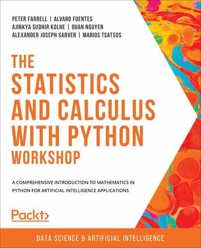
Let's take a quick example of a linear equation with two variables. Suppose the equation is y = 2x + 6. This representation is known as the slope-intercept form and has the format y = mx + c, where m is the slope and c is the y intercept of the equation.
Here, m=2 and c=6, and the line can be drawn on a graph by plotting different values of x and y:
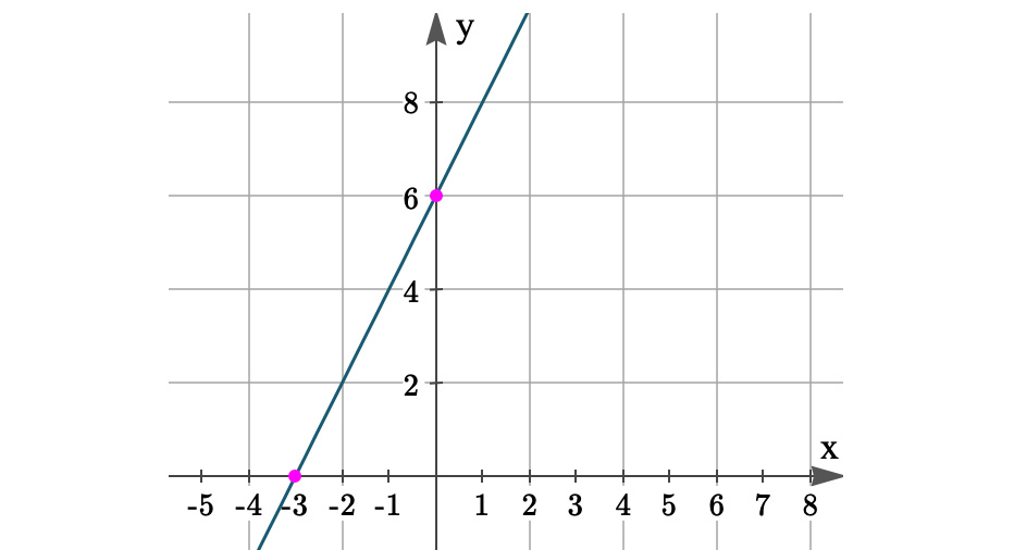
Figure 6.6: Representation of y = 2x + 6 in a 2D space
Without getting into much detail, we can imagine that there may be another line in the plane that will either be parallel to the line or will intersect this line. The linear equations intend to find the intersecting point of these lines and, based on the value of the intersecting common point, find the values of the variables x and y. As the number of dimensions increase, it becomes difficult to visualize, but fundamentally, the concept remains the same. Matrices greatly simplify the process of solving these equations. There are typically two matrices, one that contains the coefficient of x and y, and the other containing the variables x and y. Their dot product yields the resultant matrix, which is the constant or the y intercept mentioned previously. It is fairly easy to understand once we look at a quick exercise.
Exercise 6.03: Use of Matrices in Performing Linear Equations
We will now solve a linear equation problem using matrices.
John is out of town for three days and in a mood to spend until he exhausts his resources. He has three denominations of currency with him. On the first day, John spends $435 on the latest electronic tablet that he likes, on which he spends 37 of type a denomination, 20 of type b, and 12 of type c. On the second day, he goes skydiving and spends 15, 32, and 4 of denominations a, b, and c, respectively, a total of $178. On the third day, with whatever amount he is left with, he decides to go to the theatre, which costs $70, and he shells out 5, 40, and 2 of the a, b, and c denominations, respectively. Can you tell what the values of the respective denominations are?
Looking at the problem, we can tell that there are three equations and three unknown variables that we need to calculate.
- Let's put the values we know for three days in a matrix using NumPy arrays:
import numpy as np
# Input
z = np.array([[37, 20, 12],
[15, 32, 4],
[5, 40, 2]])
We now have the matrix that we need to work with. There are a few ways to solve this. In essence, this is what we need to do:
Ax = b
Where A is the matrix whose values we know, x is the matrix with unknown variables, and b is the resultant matrix.
- The resultant b matrix will be as follows. These are the amounts that John spent on the three given days:
r = np.array([[435],[178],[70]])
There are a couple of ways to solve this problem in Python:
Method 1: Finding x by doing x = A-1b:
- Let's first calculate the inverse of matrix A with the help of the function we learned earlier:
print(np.linalg.inv(z))
Note
We will be using a dot product of the matrix and not pure multiplication, as these are not scalar variables.
The output is as follows:
[[-0.06282723 0.28795812 -0.19895288]
[-0.0065445 0.0091623 0.02094241]
[ 0.28795812 -0.90314136 0.57853403]]
It is not necessary here to understand this matrix as it is just an intermediary step.
- Then, we take the dot product of the two matrices to produce a matrix, X, which is our output:
X = np.linalg.inv(z).dot(r)
print(X)
The output will be as follows:
[[10. ]
[ 0.25]
[ 5. ]]
Method 2: Using in-built methods in the linalg package:
- This same thing can be done even more easily with the help of another NumPy function called solve(). Let's name the output variable here as y.
y = np.linalg.solve(z,r)
print(y)
This produces the following output:
[[10. ]
[ 0.25]
[ 5. ]]
And in a single line, we were able to solve the linear equation in Python. We can extrapolate and comprehend how similar equations with a large number of unknown variables can be easily solved using Python.
Thus, we can see that the output after using both methods 1 and 2 is the same, which is $10, 25 cents, and $5, which are the respective denominations that we were trying to establish.
What if we were receiving the information about John's expenses iteratively instead of in one go?
- Let's first add the information that we received about John's expenses:
a = np.array([[37, 20, 12]])
- Then, let's also add the information received relating to John's other two expenses:
b = np.array([[15, 32, 4]])
c = np.array([[5, 40, 2]])
- We can easily bind these arrays together to form a matrix using the concat() function:
u = np.concatenate((a, b, c), axis=0)
print(u)
This produces the following output:
[[37 20 12]
[15 32 4]
[ 5 40 2]]
[Finished in 0.188s]
This was the same input that we used for the preceding program.
Again, if we have a lot more of these, we might apply loops to form a larger matrix, which we can then use to solve the problem.
Note
To access the source code for this specific section, please refer to https://packt.live/3eStF9N.
You can also run this example online at https://packt.live/38rZ6Fl.
Transition Matrix and Markov Chains
Now, we will be looking at one of the applications of matrices, which is a field of study all by itself. Markov chains make use of transition matrices, probability, and limits to solve real-world problems. The real world is rarely as perfect as the mathematical models we create to solve them. A car may want to travel from point A to B, but distance and speed prove insufficient parameters in reality. A cat crossing the street may completely alter all the calculations that were made to calculate the time traveled by the car. A stock market may seem to be following a predictable pattern for a few days, but overnight, an event occurs that completely crashes it. That event may be some global event, a political statement, or the release of company reports. Of course, our development in mathematical and computational models has still not reached the place where we can predict the outcome of each of these events, but we can try and determine the probability of some event happening more than others. Taking one of the previous examples, if the company reports are to be released on a particular date, then we can expect that a particular stock will be affected, and we can model this according to market analysis done on the company.
Markov chains are one such model, in which the variable depending on the Markov property takes into account only the current state to predict the outcome of the next state. So, in essence, Markov chains are a memoryless process. They make use of transition state diagrams and transition matrices for their representations, which are used to map the probability of a certain event occurring given the current event. When we call it a memoryless process, it is easy to confuse it with something that has no relation to past events, but that is not actually the case. Things are much easier to understand when we take an example to illustrate how they work. Before we jump into using Markov chains, let's first take a deeper look at how transition states and matrices work and why exactly they are used.
Fundamentals of Markov Chains
To keep things simple, let's break the concepts down into pieces and learn about them iteratively from the information that we have before we can put them together to understand the concepts.
Stochastic versus Deterministic Models
When we are trying to solve real-world problems, we often encounter situations that are beyond our control and that are hard to formulate. Models are designed to emulate the way a given system functions. While we can factor in most of the elements of the system in our model, many aspects cannot be determined and are then emulated based on their likelihood of happening. This is where probability comes into the picture. We try and find the probability of a particular event happening given a set of circumstances. There are two main types of models that we use, deterministic and stochastic. Deterministic models are those that have a set of parameter values and functions and can form a predictable mathematical equation and will provide a predictable output. Stochastic models are inclusive of randomness, and even though they have initial values and equations, they provide quantitative values of outcomes possible with some probability. In stochastic models, there will not be a fixed answer, but the likelihood of some event happening more than others. Linear programming is a good example of deterministic models, while weather prediction is a stochastic model.
Transition State Diagrams
Broadly, these form the basis for object-oriented programming, where you can describe all possible states that object can have based on given events and conditions. The state is that of the object at a given moment in time when a certain previous condition is met. Let's illustrate this with an example:
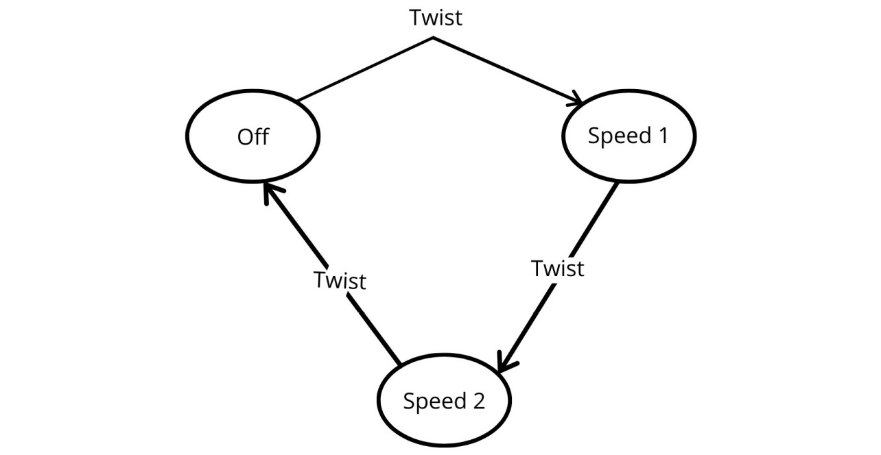
Figure 6.7: State transition diagram for a fan
This is the state transition diagram for the regulator of a table fan, which usually changes state every time we turn it clockwise until it turns back to the Off position.
Here, the state of the table fan is changing in terms of the speed, while the action is that of twisting. In this case, it is based on events, while in some other cases it will be based on a condition being met.
Let's take an example in text generation using the Markov chain that is in line with what we are going to implement. We will recall the first two lines of a nursery rhyme:
Humpty Dumpty sat on a wall,
Humpty Dumpty had a great fall.
First, let's prepare a frequency table of all the words present in the sentence:

Figure 6.8: Frequency table of words in the rhyme
Tokens are the number of words present, while keys are unique words. Hence, the values will be as follows:
Tokens = 12
Keys = 9
We may not even require everything we learn here, but it will be important once you decide to implement more complicated problems. Every transition diagram has a start and end state, and so we will add these two states here as keys:

Figure 6.9: Frequency table of start and end states
We then prepare a state chart to show the transition from one state to the next. In this case, it requires showing which word will follow the current word. So, we will be forming pairs as follows:
Figure 6.10: Word pairs
If we condense this according to keys instead of tokens, we will see that there is more than one transition for some keywords, as follows:

Figure 6.11: More than one transition for some keywords
This is done not only to reduce the state transitions, but also to add meaning to what we are doing, which we will see shortly. The whole purpose of this is to determine words that can pair with other words. We are now ready to draw our state transition diagram.
We add all the unique keys as states, and show which states these words can transition to:
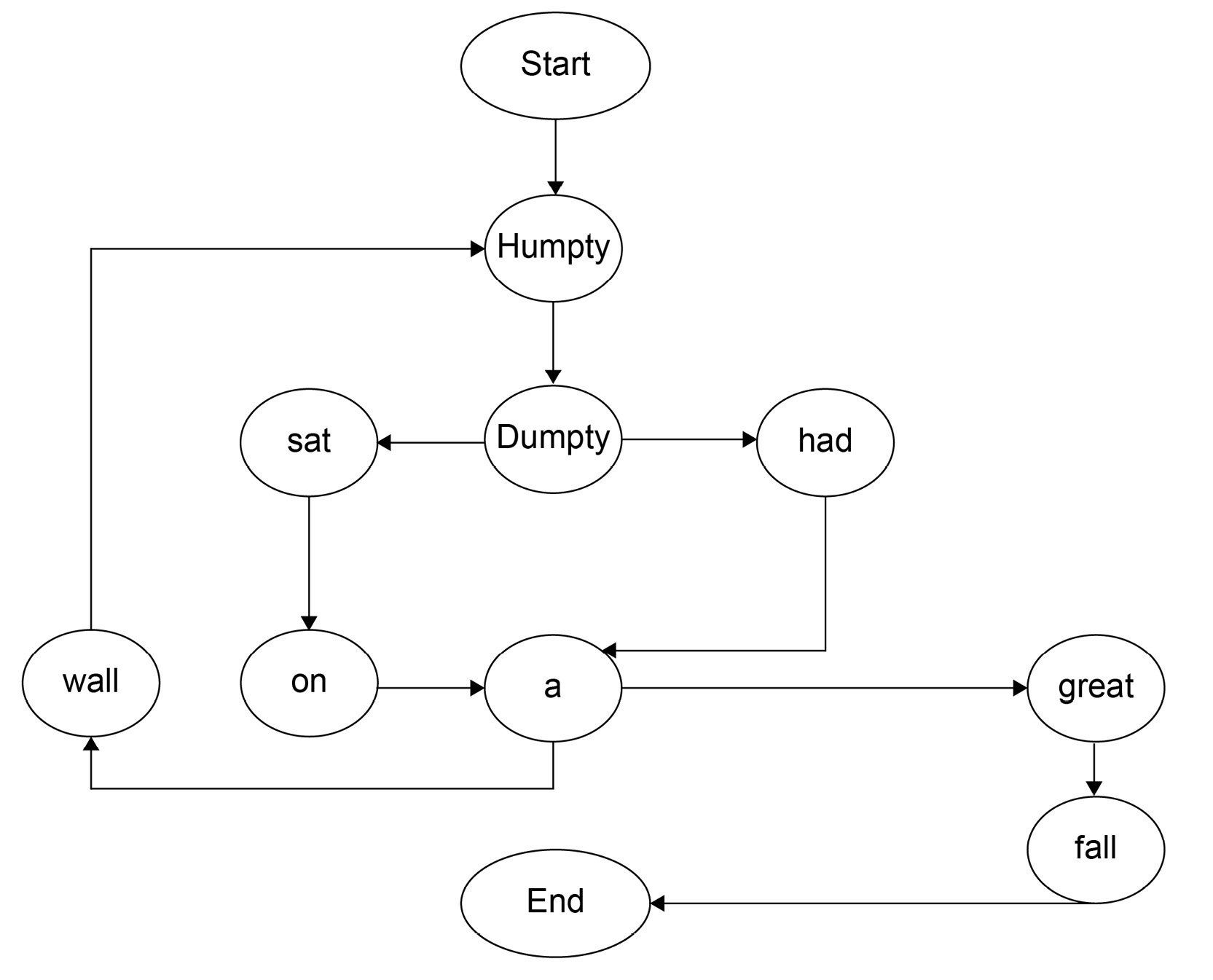
Figure 6.12: State transition diagram
If we look at the preceding diagram, we can follow any word to complete the rhyme from the set of conditions given. What remains is the probability of the keywords occurring after the given word. For that, look at the following diagram, and we can see in a fairly straightforward manner how the probability is divided between keywords according to their frequency. Note that Humpty is always followed by Dumpty, and so will have a probability of 1:
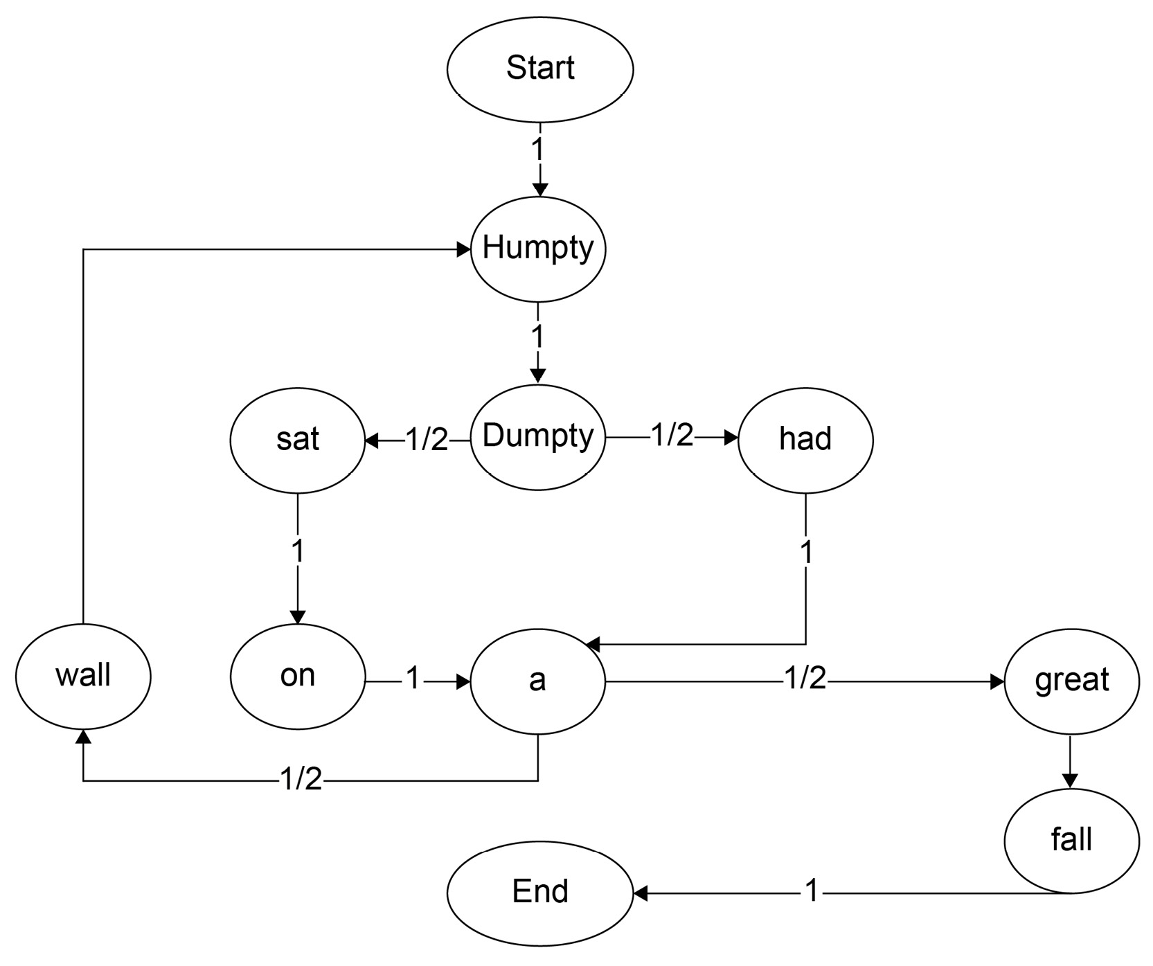
Figure 6.13: State transition diagram with probability
Now that we have discussed the state transition diagrams, we will move on to drawing transition matrices.
Transition Matrices
In the Markov process, we need to show the probability of state transitions in mathematical format for which transition matrices are used. The rows and columns are simply the states of the transition diagram. Each value in the transition matrix shows the probability of transition from one state to another. As you can imagine, many of the values in such matrices will be 0. For the problem discussed earlier, the transition matrix will have 9 states and lots of 0s. We will take a simpler example of a transition diagram and find its corresponding matrix:
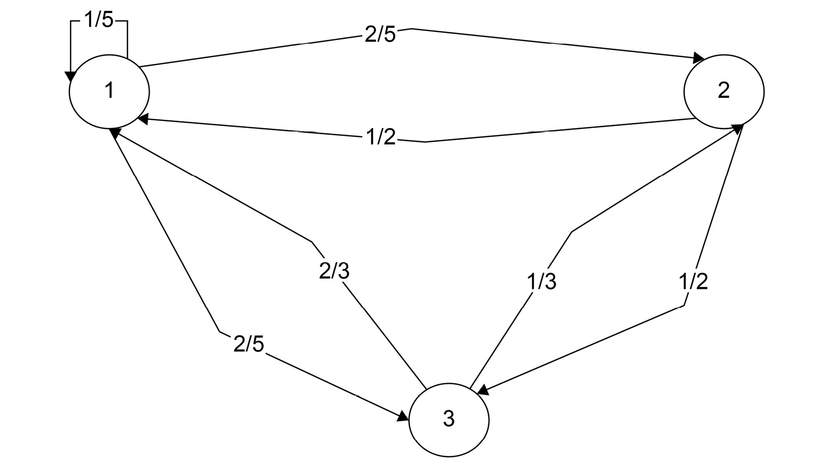
Figure 6.14: State diagram with states 1, 2, and 3
When we look at this diagram, we see the three transition states. Note that we have not included the start and end states explicitly here, but they can be necessary in certain cases. The outward arrows represent the transition from one state to the next. Once we have the diagram, it is easy to draw the matrix. Write rows and columns equal to the states of the diagram. In this case, it will be 3. Then, the 0th row will show the transition for the 1st state, the 1st row will show the second state, and so on. To generalize, each row in the matrix represents the transition probabilities of one state.
Let's first look at the matrix, and we can then discuss a couple more things:

Figure 6.15: Transition matrix
In addition to the property of rows, we can observe one more thing. The sum of all probabilities in a given row will always be equal to 1. In the first row here, the sum will be 1/5 + 2/5 + 2/5 = 5/5 = 1. This is because these states are exhaustive.
If there is no transition between two given states, the value of the states in that matrix will be 0. We can verify this by comparing the number of values present in the matrix with the number of state transitions we can see in the diagram. In this case, they are both equal to 7.
Exercise 6.04: Finding the Probability of State Transitions
Given an array containing four states, A, B, C, and D, that are randomly generated, let's find the probability of transition between these four states. We will be finding the probability of each state transition and form a transition matrix from it.
Let's generate a transition matrix in Python from a given array of inputs. We will extrapolate the same concept in the future while creating Markov chains.
- Generate an array of random states out of the characters A, B, C, and D using the random package in Python. We will then define how many elements we want by creating a constant, LEN_STR, which, in this case, we will set to 50:
# Generate random letters from 4 states A B C D
import random
tokens = []
LEN_STR = 50
for i in range(LEN_STR):
tokens.append(random.choice("ABCD"))
print(tokens)
LEN_TOKENS = len("ABCD")
This produces the following output:
['C', 'A', 'A', 'B', 'A', 'A', 'D', 'C', 'B', 'A', 'B', 'A', 'A', 'D', 'A', 'A', 'C', 'B', 'C', 'D', 'D', 'C', 'C', 'B', 'A', 'D', 'D', 'C', 'A', 'A', 'D', 'C', 'A', 'D', 'A', 'A', 'A', 'C', 'B', 'D', 'D', 'C', 'A', 'A', 'B', 'A', 'C', 'A', 'D', 'D']
Note
The use of another constant, LEN_TOKENS, which we created from the length of the string, will indicate the number of states that will be present in the problem.
- Next, we will be finding the relative values of letters and converting them into integers, primarily because integers are easier for calculations:
# Finding the relative values with ordinal values of
# ASCII characters
relative_value = [(ord(t) - ord('A')) for t in tokens]
print(relative_value)
This produces the following output:
[2, 0, 0, 1, 0, 0, 3, 2, 1, 0, 1, 0, 0, 3, 0, 0, 2, 1,
2, 3, 3, 2, 2, 1, 0, 3, 3, 2, 0, 0, 3, 2, 0, 3, 0, 0,
0, 2, 1, 3, 3, 2, 0, 0, 1, 0, 2, 0, 3, 3]
We have used cardinal values here for convenience, but we could have also done this by using a dictionary or some other method. If you are not aware, the ord() function here returns the ASCII value of characters in the string. For example, the ASCII values for A and D are 65 and 68, respectively.
- Now, find the difference between these ASCII values and put them in a list, ti. We could have also updated the token list in situ, but we are keeping them separate simply for clarity:
#create Matrix of zeros
m = [[0]*LEN_TOKENS for j in range(LEN_TOKENS)]
print(m)
# Building the frequency table(matrix) from the given data
for (i,j) in zip(relative_value, relative_value [1:]):
m[i][j] += 1
print(list(zip(relative_value, relative_value [1:])))
print(m)
This produces the following output:
[[0, 0, 0, 0], [0, 0, 0, 0], [0, 0, 0, 0], [0, 0, 0, 0]]
[(2, 0), (0, 0), (0, 1), (1, 0), (0, 0), (0, 3), (3, 2), (2, 1), (1, 0), (0, 1), (1, 0), (0, 0), (0, 3), (3, 0), (0, 0), (0, 2), (2, 1), (1, 2), (2, 3), (3, 3), (3, 2), (2, 2), (2, 1), (1, 0), (0, 3), (3, 3), (3, 2), (2, 0), (0, 0), (0, 3), (3, 2), (2, 0), (0, 3), (3, 0), (0, 0), (0, 0), (0, 2), (2, 1), (1, 3), (3, 3), (3, 2), (2, 0), (0, 0), (0, 1), (1, 0), (0, 2), (2, 0), (0, 3), (3, 3)]
[[8, 3, 3, 6], [5, 0, 1, 1], [5, 4, 1, 1], [2, 0, 5, 4]]
We have now initialized a matrix of zeros depending on the size of the LEN_TOKENS constant we generated earlier and used that to build a zero matrix.
In the second part, we are creating tuples of pairs, as we did in the earlier problem, and updating the frequency of the transition matrix according to the number of transitions between two states. The output of this is the last line in the preceding code.
Note
We are iteratively choosing to update the value of matrix m in each step instead of creating new matrices.
- We will now be generating the probability, which is merely the relative frequency in a given row. As in the first row, the transition from A to A is 8, and the total transitions from A to any state are 20. So, in this case, the probability will be 8/20 = 0.4:
# Finding the Probability
for state in m:
total = sum(state)
if total > 0:
state[:] = [float(f)/sum(state) for f in state]
The code goes like that for every row and, if the sum function is greater than 0, we find the probability. Note here that the float function is used to avoid type conversion to int in some versions of Python. Also, note the use of state[:], which creates a shallow copy and thereby prevents conflicts of type conversions internally.
- Now, let's print the state object by adding the following code:
for state in m:
print(state)
Here, we iterate through the rows in a matrix and print out the values, and this is our transition matrix.
This produces the following output:
[0.4, 0.15, 0.15, 0.3]
[0.7142857142857143, 0.0, 0.14285714285714285, 0.14285714285714285]
[0.45454545454545453, 0.36363636363636365, 0.09090909090909091, 0.09090909090909091]
[0.18181818181818182, 0.0, 0.45454545454545453, 0.36363636363636365]
Thus, we are able to construct a transition matrix for describing state transitions, which shows us the probability of transition from one state to the next. Hence, the likelihood of A finding A as the next letter is 0.4, A going to B will be 0.15, and so on.
Note
To access the source code for this specific section, please refer to https://packt.live/31Ejr9c.
You can also run this example online at https://packt.live/3imNsAb.
Markov Chains and Markov Property
Transition states and matrices essentially cover the majority of Markov chains. Additionally, there are a few more things worth understanding. As mentioned earlier, the Markov property applies when variables are dependent on just the current state for their next state. The probabilistic model formed may determine the likelihood of the outcome from the current state, but the past state is seen as independent and will not affect the result. Take a coin toss; we may create a chart of probabilities of heads or tails, but that will not determine the outcome.
The Markov property should essentially meet two criteria:
- It should only be dependent on the current state.
- It should be specific for a discrete time.
Without getting too confused, the time considered in models is either discrete or continuous. The flipping of a coin can be considered a discrete-time event because it has a definite outcome, such as heads or tails. On the other hand, weather patterns or stock markets are continuous-time events; weather, for example, is variable throughout the day and does not have a start and end time to measure when it changes. To deal with such continuous events, we require techniques such as binning to make them discrete. Binning, in simple terms, means grouping data in fixed amounts based on quantity or time. As a Markov chain is memoryless, it essentially becomes a discrete-time and state-space process.
There are special matrices that are built for specific purposes. For example, sparse matrices are extensively used in data science as they are memory- and computationally-efficient. We did not deal too much with the manipulation of elements within the matrix as that is essentially like dealing with a list of lists, but it is worthwhile spending some time on this in the future.
Other than Markov chains, there are a few more models for random processes. These include autoregressive models, Poisson models, Gaussian models, moving-average models, and so on. Each deals with the aspect of randomness differently, and there are supporting libraries in Python for almost all of them. Even within Markov chains, there are complicated topics involving multidimensional matrices or second-order matrices, Hidden Markov models, MCMC or Markov chain Monte Carlo methods, and so on. You have to make your own choice of how deep you want to go down the rabbit hole.
Activity 6.01: Building a Text Predictor Using a Markov Chain
The aim of this activity is to build our very own text predictor based on what we have learned. We will take the transcripts of a speech from a famous leader and build a text predictor based on the content of the speech using a Markov chain model and state transitions. Perform these steps to achieve the goal:
- First, find a suitable, sufficiently large transcript of a speech given by a famous person, such as a scientist or a political or spiritual leader of your choice. To get you started, a sample text with the filename churchill.txt is added to the GitHub repository at https://packt.live/38rZy6v.
- Generate a list that describes state transition by showing a correlation between a given word and the words that follow it.
- Sort through the list you have made and make a hash table by grouping the words that follow a given word in different positions. For example, these follow-up words will group to form John: [cannot, completely, thought, …]:
John cannot…, John completely…, and John thought ..,
- Use a random word generator to generate and assign a value to the first word.
- Finally, create a random generator that will create a sentence based on the transition states that we have declared.
Hints
This activity requires a few Python methods that you should be familiar with.
To get you started, you can read in the transcript from a text file using open('churchill.txt').read(), and then split it into a list of words using split().
You can then iterate through the list and append the elements to a new list, which will store the keyword and the word following it.
Then, use a dictionary to form a key-value pair for each tuple in your new list.
A random word corpus can be generated using the np.random() function.
The sentence formation comes from joining together the elements of the list that we generated.
Note
The solution to this activity can be found on page 677.
This way, we have made our own text predictor. Such a text predictor can be considered a foundational step in terms of the vast and fast-growing field of text generators. It is far from perfect; there are several reasons for this, some of which are as follows:
- The text sample that we have chosen is usually many times larger than the one we have chosen. Our text contains about 22,000 words while, in practice, millions of words are fed as data.
- There is a lot better moderation in terms of the stop words, punctuation, and beginning/ending of sentence formations using the proper rules of NLP that is not applied here.
- We have used a simple random generator to select our words, while actual models use probability and statistical models to generate significantly more accurate outputs.
Having said that, we have completed our first text predictor, and more complicated text predictors are fundamentally based on the way we have described them.
Though by no means can this be considered smooth, we have still written our first text predictor with just a few lines of code, and that is a great start.
Summary
In this chapter, we were able to cover the topic of matrices, which is fundamental to a number of topics, both in mathematics and in using Python. Data science today is primarily based on the efficient use of matrices. We studied their application in the form of Markov chains and, although an important topic, there is no dearth of topics to explore that come under the umbrella of applications using matrices.
Next, we will delve into the world of statistics. We will use a more formal and systematic approach in first understanding the building blocks of statistics, then understanding the role of probability and variables, and finally tying these concepts together to implement statistical modeling.
YKA34
LHL39