Overview
In this chapter, you will learn to calculate the derivatives of functions at a given value of x. You'll also learn to calculate the integrals of functions between given values and use derivation to solve optimization problems, such as maximizing profit or minimizing cost. By the end of this chapter, you will be able to use calculus to solve a range of mathematical problems.
Introduction
Calculus has been called the science of change, since its tools were developed to deal with constantly changing values such as the position and velocity of planets and projectiles. Previously, there was no way to express this kind of change in a variable.
The first important topic in calculus is the derivative. This is the rate of change of a function at a given point. Straight lines follow a simple pattern known as the slope. This is the change in the y value (the rise) over a given range of x values (the run):
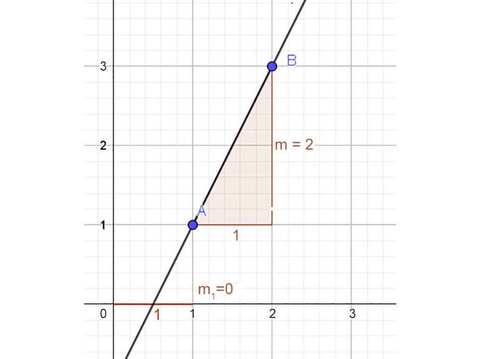
Figure 10.1: Slope of a line
In Figure 10.1, the y value in the line increases by 2 units for every 1-unit increase in the x value, so we divide 2 by 1 to get a slope of 2.
However, the slope of a curve isn't constant over the whole curve like it is in a line. So, as you can see in Figure 10.2, the rate of change of this function at point A is different from the rate of change at point B:
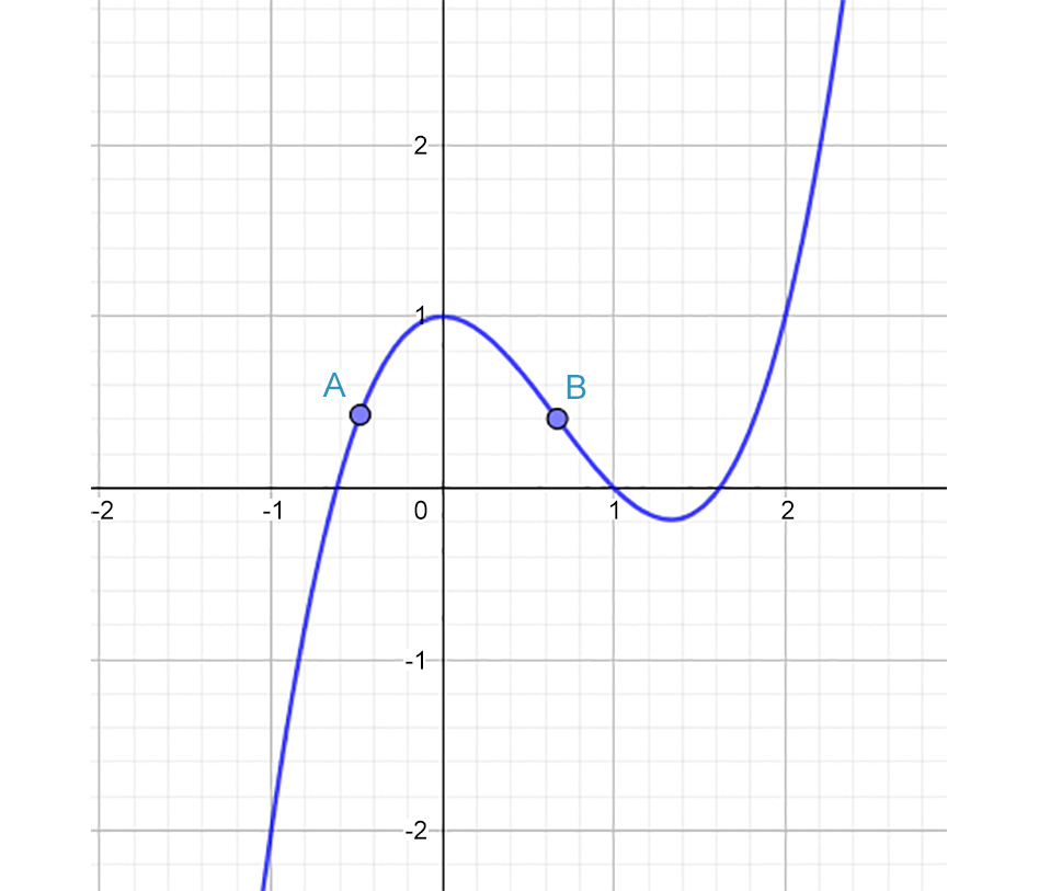
Figure 10.2: Finding the slope of a curve
However, if we zoom in closely enough on point A, we see the curve is pretty closely approximated by a straight line.

Figure 10.3: Zooming in on the curve
This is how derivatives work: we make the change in x, the run, small enough that the slope over that small part of the curve will closely approximate the rate of change of the curve at that point. Let's see what it looks like in Python.
Writing the Derivative Function
For all the fear whipped up about derivatives in calculus courses, the function for calculating a derivative numerically is surprisingly easy.
In a Jupyter notebook, we'll define a function, f(x), to be the parabola y = x2:
def f(x):
return x**2
Now we can write a function to calculate the derivative at any point (x, f(x)) using the classic formula:

Figure 10.4: Formula for calculating derivatives
The numerator is the rise and the denominator is the run. Δ x means the change in x, and we're going to make that a really small decimal by dividing 1 by a million:
def f(x):
return x**2
def derivative(f,x):
"""
Returns the value of the derivative of
the function at a given x-value.
"""
delta_x = 1/1000000
return (f(x+delta_x) - f(x))/delta_x
Note
The triple-quotes ( """ ) shown in the code snippet below are used to denote the start and end points of a multi-line code comment. Comments are added into code to help explain specific bits of logic.
Now we can calculate the derivative of the function at any x value and we'll get a very accurate approximation:
for i in range(-3,4):
print(i,derivative(f,i))
If you run the preceding code, you'll get the following output:
-3 -5.999999000749767
-2 -3.999998999582033
-1 -1.999999000079633
0 1e-06
1 2.0000009999243673
2 4.0000010006480125
3 6.000001000927568
These values are only a little off from their actual values (-5.999999 instead of -6). We can round up the printout to the nearest tenth and we'll see the values more clearly:
for i in range(-3,4):
print(i,round(derivative(f,i),1))
The output will be:
-3 -6.0
-2 -4.0
-1 -2.0
0 0.0
1 2.0
2 4.0
3 6.0
We've calculated the derivative of the function y = x2 at a number of points and we can see the pattern: the derivative is always twice the x value. This is the slope of the line that approximates the curve at that point. The awesome power of this method will become clear in this exercise.
Exercise 10.01: Finding the Derivatives of Other Functions
We can use our derivative function to calculate the derivative of any function we can express. There's no need to go through tedious algebraic manipulations when we can simply use the tiny run method of calculating the slope. Here, our function will find the derivative of some complicated-looking functions. We reused f, but you can call other functions as well. In this exercise, you will find the derivatives of each function at the given x values:

Figure 10.5: Function definitions at given x values
Perform the following steps:
- First, we'll need to import the square root function from the math module:
from math import sqrt
- Here are the preceding functions in the equations, translated into Python code:
def f(x):
return 6*x**3
def g(x):
return sqrt(2*x + 5)
def h(x):
return 1/(x-3)**3
- Define the derivative function if you haven't already:
def derivative(f,x):
"""Returns the value of the derivative of
the function at a given x-value."""
delta_x = 1/1000000
return (f(x+delta_x) - f(x))/delta_x
- Then print out the derivatives by calling each function and the desired x value:
print(derivative(f,-2),derivative(g,3),derivative(h,5))
The output will be as follows:
71.99996399265274 0.30151133101341543 -0.18749981253729509
You've just learned a very important skill: finding the derivative of a function (any function) at a specific x value. This is the reason calculus students do lots of hard algebra: to get the derivative as a function, and then they can plug in an x value. However, with Python, we just directly calculated the numerical derivative of a function without doing any algebra.
Note
To access the source code for this specific section, please refer to https://packt.live/2AnlJOC.
You can also run this example online at https://packt.live/3gi4I7S.
Finding the Equation of the Tangent Line
A common question in calculus is to find the equation of the line tangent to the curve at a given point. Remember our points A and B? The tangent lines are the lines that closely approximate the curve at those points, as you can see in Figure 10.6:
Figure 10.6: Two tangent lines to a curve
Let's use the information in Figure 10.6. The equation is as follows:

Figure 10.7: Equation of f(x)
The x value at point A in Figure 10.6 is -0.48 and the x value at B is 0.67. The great thing about using Python to do this is it won't matter if the given values are whole numbers, negatives, or decimals, the computer will easily process the number-crunching.
To find the equation of a line, all we need is a slope and a point. If you remember your algebra, you can use this formula:

Figure 10.8: Equation of a line
We're given the function and the point (x0, y0), so from that, we can find the slope m from the derivative of the function at the given x value. The equation of the tangent line will be in the form y = mx + b, and the only thing we don't know is b, the y intercept of the line. But if we rearrange the preceding equation, we can see it on the right side of the equation:

Figure 10.9: Equation of line at the point
We need to find the slope m using the derivative function we already have, then plug it into y0 - m x0. To do this, perform the following steps:
- First, we'll define our f(x) function:
def f(x):
return x**3 - 2*x**2 + 1
- Then we'll write a function to return the y intercept of a line given the slope and a point. Call it point_slope:
def point_slope(m,x,y):
"""Finds the y-intercept of a line
given its slope m and a point (x,y)"""
return y-m*x
- Finally, we'll write a function that takes the function f and an x value and finds the derivative of f at x, puts that into the point_slope function, and prints out the equation of the line in y = mx + b form. Call it tangent_line:
def tangent_line(f,x):
"""Finds the equation of the line
tangent to f at x."""
- We find the slope of the tangent line by taking the derivative of f at x:
m = derivative(f,x)
- Then we use the point_slope function to find the y intercept:
y0 = f(x)
b = point_slope(m,x,y0)
print("y = ",round(m,2),"x + ",round(b,2))
- Now, to get the equations of the lines tangent to f at x = -0.48 and x = 0.67, use the following code:
for x in [-0.48,0.67]:
tangent_line(f,x)
The output is as follows:
y = 2.61 x + 1.68
y = -1.33 x + 1.3
In this section, we learned how to find out the equations of tangent lines at specific values of x.
Calculating Integrals
One major topic of calculus is differential calculus, which means taking derivatives, as we've been doing so far in this chapter. The other major topic is integral calculus, which involves adding up areas or volumes using many small slices.
When calculating integrals by hand, we're taught to reverse the algebra we would do to find a derivative. But that algebra gets messy and, in some cases, impossible. The hard version we learned in school was Riemann sums, which required us to cut the area under a curve into rectangular slices and add them up to get the area. But you could never work with more than 10 slices in a realistic amount of time, certainly not on a test.
However, using Python, we can work with as many slices as we want, and it saves us the drudgery of jumping through a lot of hoops to get an algebraic equation. The point of finding the algebraic equation is to obtain accurate number values, and if using a program will get us the most accurate numbers, then we should definitely take that route.
Figure 10.10 shows a function and the area under it. Most commonly the area is bounded by the function itself, a lower x value a, an upper x value b, and the x axis.

Figure 10.10: The area S under a curve defined by the function f(x) from a to b
What we're going to do is to slice the area S into rectangles of equal width, and since we know the height (f(x)), it'll be easy to add them all up using Python. Figure 10.11 shows what the situation looks like for f(x) = x2:

Figure 10.11: The area S sliced into 10 rectangles of equal width
First, we'll define the function and choose the number of rectangles (so that the value of both will be easy to change). In this instance, we will use 20 rectangles, which will give us a higher degree of accuracy than the 10 rectangles shown in Figure 10.11:
def f(x):
return x**2
number_of_rectangles = 20
Then we define our integral function. First, divide the range (b – a) into equal widths by dividing by num, the number of rectangles:
def integral(f,a,b,num):
"""Returns the sum of num rectangles
under f between a and b"""
width = (b-a)/num
Then we'll loop over the range, adding the area of the rectangles as we go. We do this with a one-line list comprehension. For every n, we multiply the base of the rectangle (width) by the height (f(x)) to get the area of each rectangle. Finally, we return the sum of all the areas:
area = sum([width*f(a+width*n) for n in range(num)])
return area
This is how the function call looks:
for i in range(1,21):
print(i,integral(f,0,1,i))
The output shows how, with more rectangles, we get closer and closer to the actual value of the area:
1 0.0
2 0.125
3 0.18518518518518517
4 0.21875
5 0.24000000000000005
6 0.2546296296296296
7 0.26530612244897955
8 0.2734375
9 0.279835390946502
10 0.2850000000000001
11 0.2892561983471075
12 0.292824074074074
13 0.2958579881656805
14 0.29846938775510196
15 0.30074074074074075
16 0.302734375
17 0.3044982698961938
18 0.3060699588477366
19 0.3074792243767312
20 0.3087500000000001
It seems to be growing slowly. What if we jump ahead to 100 rectangles? That would create the situation shown in Figure 10.12:

Figure 10.12: Smaller rectangles making a better approximation of the area
Here's how we change the print statement to give us the area of the 100 rectangles:
print(100,integral(f,0,1,100))
The output will be as follows:
100 0.32835000000000014
How about 1,000 rectangles, an integral that would be extremely difficult and time-consuming to calculate by hand? Using Python, we'll just change 100 to 1000 and get a much more accurate approximation:
print(1000,integral(f,0,1,1000))
The output will be as follows:
1000 0.33283350000000034
And summing up 100,000 rectangles gets us 0.3333283333. It seems like it's getting close to 0.333, or 1/3. But adding more zeroes doesn't cost us anything, so feel free to increase the number of rectangles as much as required to get a more accurate result.
Using Trapezoids
We can get better approximations sooner using trapezoids rather than rectangles. That way, we won't miss as much area, as you can see in Figure 10.13:

Figure 10.13: Using trapezoids for better approximations to the curve
The following is the formula for the trapezoidal rule:

Figure 10.14: Formula for area of trapezoids
The heights of the segments at the endpoints x = a and x = b are counted once, while all the other heights are counted twice. That's because there are two heights in the formula for the area of a trapezoid. Can you guess how to adapt your integral function to be trapezoidal?
def trap_integral(f,a,b,num):
"""Returns the sum of num trapezoids
under f between a and b"""
width = (b-a)/num
area = 0.5*width*(f(a) + f(b) + 2*sum([f(a+width*n) for n in range(1,num)]))
return area
Now we'll run the trap_integral function using 5 trapezoids:
print(trap_integral(f,0,1,5))
The output will be as follows:
0.3400000000000001
So, by using only 5 trapezoids, we have reduced the error to 3%. (Remember, we know the true value of the area for this function is 0.333...) Using 10 trapezoids, we get 0.335, which has an error of 0.6%.
Exercise 10.02: Finding the Area Under a Curve
In this exercise, we'll find the area under the following functions in the given intervals:
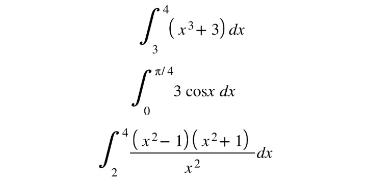
Figure 10.15: Formula for intervals
Perform the following steps to find the area. Having written the trap_integral function to use trapezoids to approximate the area under a curve, it's easy: just define the function (you may have to import a trig function and pi) and declare the endpoints. Have it use 100 trapezoids, because that'll be very accurate and quickl:
- First, import the math functions you'll need and define f, g, and h:
from math import cos,pi
def f(x):
return x**3 + 3
def g(x):
return 3*cos(x)
def h(x):
return ((x**2 - 1)*(x**2+1))/x**2
- Then call the trap_integral function on each function between the specified x values:
print(trap_integral(f,3,4,100))
print(trap_integral(g,0,pi/4,100))
print(trap_integral(h,2,4,100))
The output is as follows:
46.75017499999999
2.1213094390731206
18.416792708494786
By now, you can probably see the power in this numerical method. If you can express a function in Python, you can get a very accurate approximation of its integral using the function for adding up all the rectangles under the curve, or even more accurately, the function for adding up all the trapezoids under the curve.
Note
To access the source code for this specific section, please refer to https://packt.live/3dTUVTG.
You can also run this example online at https://packt.live/2Zsfxxi.
Using Integrals to Solve Applied Problems
If a curve is rotated about the x or y axis or a line parallel to one of the axes, to form a 3D object, we can calculate the volume of this solid by using the tools of integration. For example, let's say the parabola y = x2 is rotated around its axis of symmetry to form a paraboloid, as in Figure 10.16:
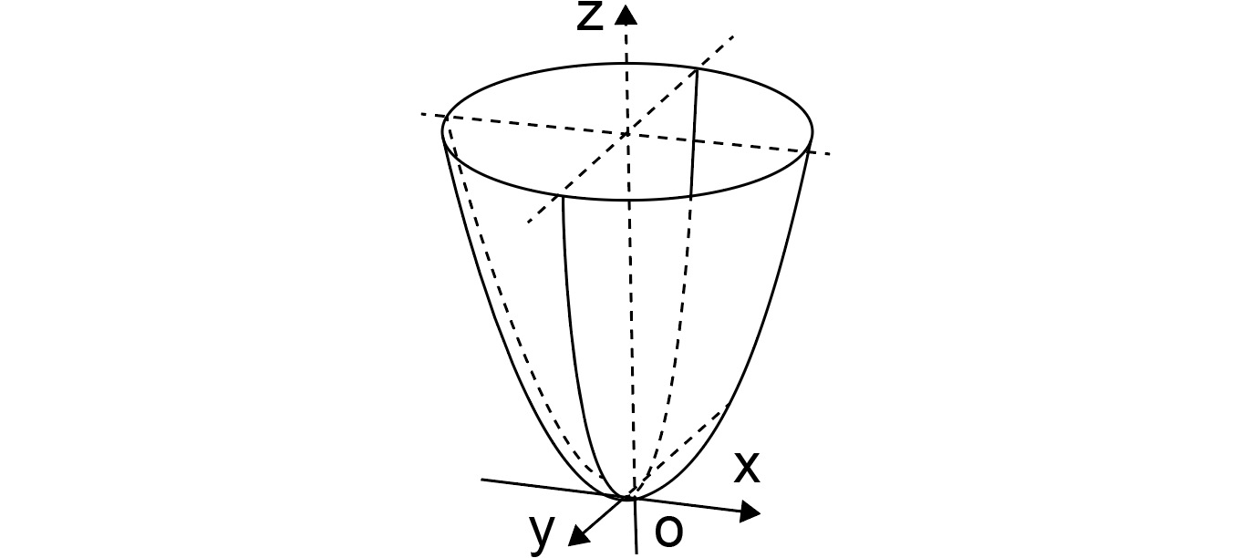
Figure 10.16: A parabola rotated about the z axis
We can find the volume by adding up all the slices of the paraboloid as you go up the solid. Just as before, when we were using rectangles in two dimensions, now we're using cylinders in three dimensions. In Figure 10.16, the slices are going up the figure and not to the right, so we can flip it in our heads and redefine the curve y = x2 as y = sqrt(x).
Now the radius of each cylinder is the y value, and let's say we're going from x = 0 to x = 1:
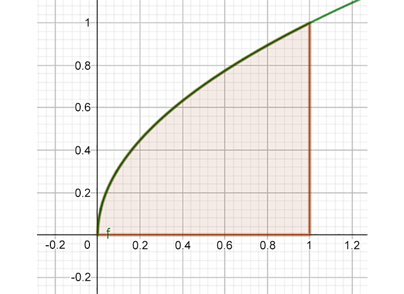
Figure 10.17: Flipping the paraboloid on its side
The endpoints are still 0 and 1, but the radius of the curve is the y value, which is sqrt(x). So the volume of each circular slice is the volume of a cylinder (pi * radius2 * height), in this case pi * r2 * thickness, or pi * sqrt(x)2 * width.
First, we import sqrt and pi from the math module and define f(x):
from math import sqrt, pi
def f(x):
return sqrt(x)
Then we'll define a function that will take the function of the paraboloid and the beginning and ending values of x. It starts off by defining the running volume and the number of slices we're going to use:
def vol_solid(f,a,b):
volume = 0
num = 1000
Then we calculate the thickness of the slices by dividing the range of x values by the number of slices:
width = (b-a)/num
Now we calculate the volume of each cylindrical slice, which is pi * r2 * width. We add that to the running volume, and when the loop is done we return the final volume:
for i in range(num):
# volume of cylindrical disk
vol = pi*(f(a+i*width))**2*width
volume += vol
return volume
Let's add up all the volumes between 0 and 1:
print(vol_solid(f,0,1))
The output will be as follows:
1.5692255304681022
This value is an approximation of the volume of the bounded paraboloid. Again, the more slices we split the function up into, the more accurate the approximation to the real volume.
Exercise 10.03: Finding the Volume of a Solid of Revolution
Here's another solid-of-revolution problem: find the volume of the solid formed when the following functions are rotated around the x axis on the given intervals.
In the following figure, the green curve is f(x) = 4 – 4x2 and the red curve is g(x) = 1-x2. Find the volume of the solid formed when the area between the functions is rotated about the x axis.
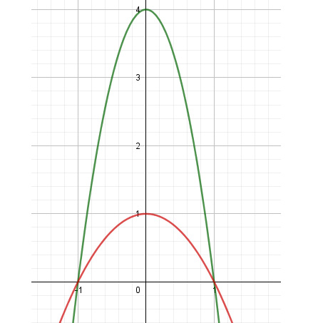
Figure 10.18: A two-dimensional look at the two functions
The resulting shape of the solid would be as follows:
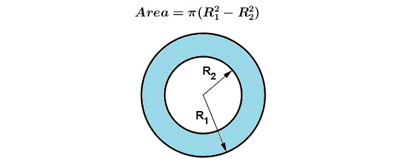
Figure 10.19: The resulting shape is like a ring
This is like a problem of finding the area of a ring, as shown in the preceding figure. The formula is as follows:

Figure 10.20: Formula for area of a ring
Now to find the volume of the solid using Python, perform the following steps:
- Create f and g as usual, and a third function (h) to be the difference of the squares of f and g, from the ring area formula:
def f(x):
return 4 -4*x**2
def g(x):
return 1-x**2
def h(x):
return f(x)**2-g(x)**2
- Now the volume of the solid will be the sum of a given number (num) of cylinders made between the functions. We do the same thing as in our integration function. The radius of the cylinder is the same as the height of our rectangle when we were integrating:
def vol_solid(f,a,b):
volume = 0
num = 10000
width = (b-a)/num
for i in range(num):
- The volume of a cylinder is pi*r2*h, and we'll add that to the running total volume:
vol = pi*(f(a+i*width))*width
volume += vol
return volume
- Here's where we call vol_solid on the h function for x between -1 and 1:
print(vol_solid(h,-1,1))
The output will be as follows:
50.26548245743666
Hence, the volume of the resulting solid is 50.3 cubic units. So, we have used our function to find the volumes of solids, and we have adapted it to find the volume of the solid between two curves.
Note
To access the source code for this specific section, please refer to https://packt.live/2NR9Svg.
You can also run this example online at https://packt.live/3eWJaxs.
Using Derivatives to Solve Optimization Problems
In many applied problems, we're looking for an optimal point, where the error is lowest, for example, or the profit is highest. The traditional way is to model the situation using a function, find the derivative of the function, and solve for the input that makes the derivative zero. This is because the derivative is zero at local minima and maxima, as shown in the following figure:
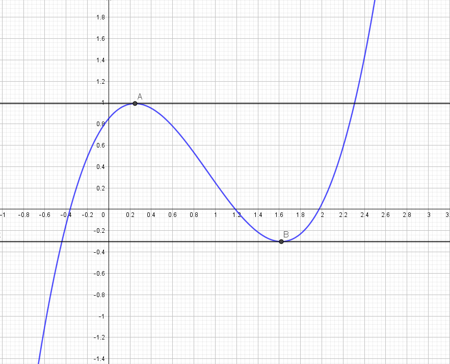
Figure 10.21: A cubic function and the points we want to find
The function we're given in the figure is f(x) = x3 - 2.8x2 + 1.2x + 0.85. We're interested in finding the local maximum, point A, and the local minimum, point B. We would have to differentiate the function and solve the resulting equation by hand. But using a computer, we can simply start at a value of x on the left of the grid and take small steps, checking f(x) until we get a change in direction. To do that, we can use our derivative function to check when the derivative changes sign.
First, we define f(x):
def f(x):
return x**3-2.8*x**2+1.2*x+0.85
Then we'll define a function called find_max_mins to start at a minimum x value and take tiny steps, checking if the derivative equals zero or if it changes sign, from positive to negative or vice versa. The most mathematical way to do that is to check whether the previous derivative times the new one is negative:
def find_max_mins(f,start,stop,step=0.001):
x = start
deriv = derivative(f,x)
while x < stop:
x += step
#take derivative at new x:
newderiv = derivative(f,x)
#if derivative changes sign
if newderiv == 0 or deriv*newderiv < 0:
print("Max/Min at x=",x,"y=",f(x))
#change deriv to newderiv
deriv = newderiv
Finally, we call the function so it'll print out all the values at which the derivative changes sign:
find_max_mins(f,-100,100)
The output is as follows:
Max/Min at x= 0.247000000113438 y= 0.9906440229999803
Max/Min at x= 1.6200000001133703 y= -0.3027919999998646
These are the local maximum and local minimum of f in Figure 10.21.
Exercise 10.04: Find the Quickest Route
We can use this procedure of finding maxima and minima to find the minimum value of a complicated function. In traditional calculus classes, students have to take the derivative algebraically, set it to zero, and then solve the resulting equation. We can model the situation in Python and use our derivative and the find_max_min functions to easily find the minimum value. Here's the situation: a lighthouse is located 6 kilometers offshore, and a cabin on the straight shoreline is 9 kilometers from the point on the shore nearest the lighthouse. If you row at a rate of 3 km/hr and walk at a rate of 5 km/hr, where should you land your boat in order to get from the lighthouse to the cabin as quickly as possible?
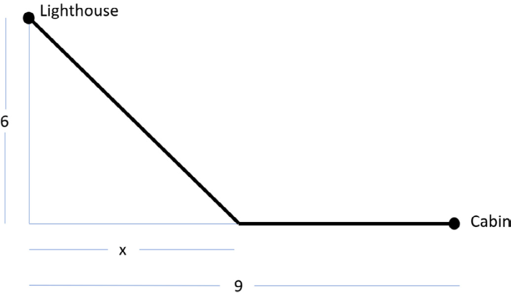
Figure 10.22: Distance of the lighthouse from the cabin
Perform the following steps to complete the exercise:
- We're aiming to minimize the time it takes to make this trip, so let's make a formula for time. Remember, time is distance divided by rate:

Figure 10.23: Formula for calculating time
- And there's the function we need to minimize. The optimal x is going to be between 0 and 9 kilometers, so we'll set those as our start and end values when we call our find_max_mins function:
from math import sqrt
def t(x):
return sqrt(x**2+36)/3 + (9-x)/5
find_max_mins(t,0,9)
The output will be as follows:
Max/Min at x= 4.4999999999998375 y= 3.4000000000000004
That's very close to 4.5 kilometers along the beach. This is a very useful calculation: we found the shortest distance between two points when other constraints have been put in place.
Note
To access the source code for this specific section, please refer to https://packt.live/31DwYxu.
You can also run this example online at https://packt.live/38wNRM5.
Exercise 10.05: The Box Problem
There's a classic problem given to all calculus students in which a manufacturer has a rectangular piece of material that they want to make into a box by cutting identical squares out of the corners, like in the following figure:

Figure 10.24: Cutting squares out of the corners of a rectangle
In this case, the piece of material is 10 inches by 12 inches. Here's the problem: find the size of the square to cut out in order to maximize the volume of the resulting box:
- The formula for the volume of the box will be length multiplied by width multiplied by height. In terms of x, the length of the square cut from the corners, the length of the box is 12 – 2x, since two corners are cut out of the 12-inch sides. Similarly, the width of the box will be 10 – 2x. The height, once the "flaps" are bent upwards, will be x. So, the volume is:

Figure 10.25: Formula to calculate the volume
- Here's how you define this function in Python:
def v(x):
return x*(10-2*x)*(12-2*x)
- By now, you know how to put this into your find_max_mins function. We only want to plug in values between 0 and 5 because more than 5 inches would mean we'd be left with no side (the width is 10 inches):
find_max_mins(v,0,5)
The output will be as follows:
Max/Min at x= 1.8109999999999113 y= 96.77057492400002
The maximum volume is achieved by cutting squares with side length 1.81 inches. Here's a plot of the volume:
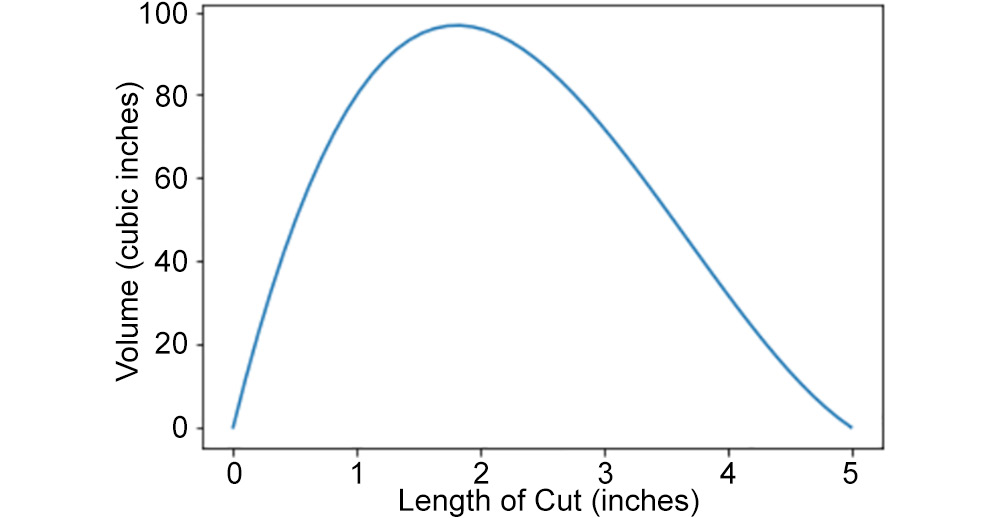
Figure 10.26: Plot of maximum value achieved
We can see that the maximum volume is achieved when a square of 1.81 inches is cut from each side, since this is where the maximum point of the plot lies.
Note
To access the source code for this specific section, please refer to https://packt.live/3gc11AC.
You can also run this example online at https://packt.live/2NNSNmb.
Exercise 10.06: The Optimal Can
A cylindrical can hold 355 cm3 of soda. What dimensions (radius and height) will minimize the cost of metal to construct the can? You can neglect the top of the can:
- The surface area of a cylinder is the area of the bottom (a circle, so πr2) plus the area of its side, which is a rectangle of base 2πr and a height of h. The volume of a cylinder is πr2h, so we put it all together:

Figure 10.27: Formula to calculate the volume of a cylinder
- The volume is already set to 355. From there, we can get an expression for h in terms of r and we'll have the surface area all in terms of one variable:
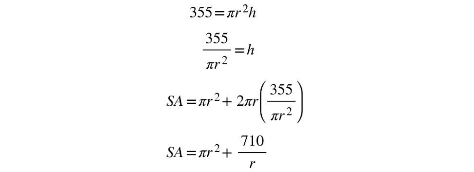
Figure 10.28: Substituting the values in the formula
- Let's express it in Python and put it in our find_max_mins function:
from math import pi
def surf_area(r):
return pi*r**2 + 710/r
find_max_mins(surf_area,0.1,10)
When you run the code, the output will be as follows:
Max/Min at x= 4.834999999999949 y= 220.28763352297025
So the solution is for the radius to be around 4.8 cm and the height to be 355/(π(4.8)2) = 4.9 cm. That means the can is about twice as wide as it is tall. Here's a plot of the surf_area function for cans between 2 and 6 cm. You can see the point that minimizes the material, between 4.5 and 5 cm. We calculated it to be exactly 4.9 cm:
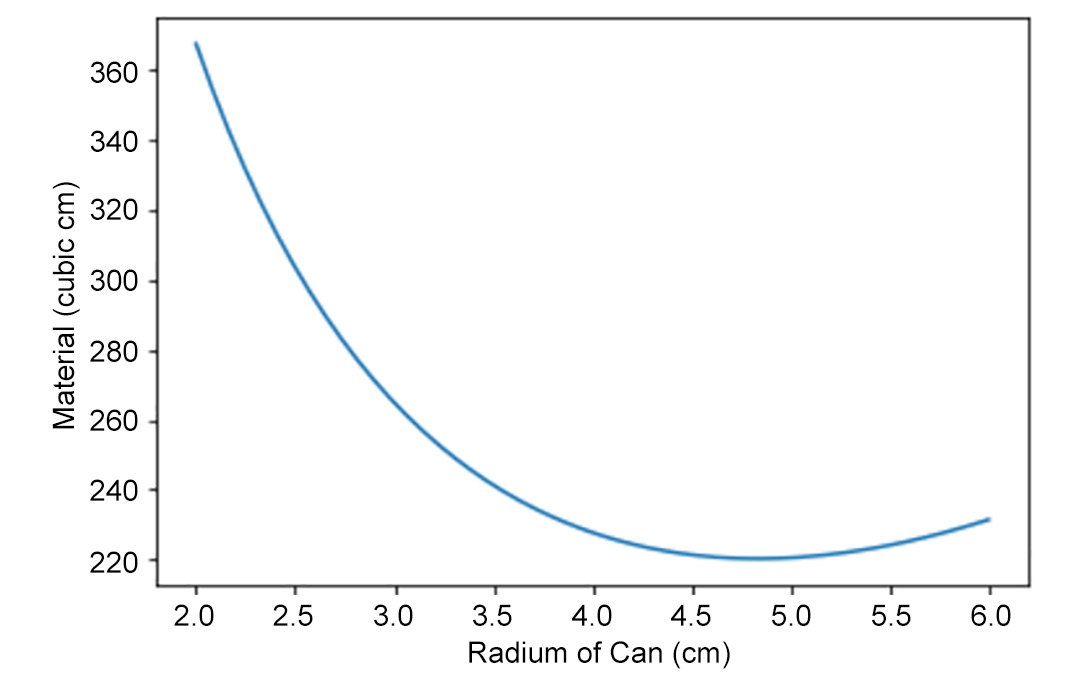
Figure 10.29: Finding the minimum material needed to make a can
Note
To access the source code for this specific section, please refer to https://packt.live/2Zu2bAK.
You can also run this example online at https://packt.live/38lUNeE.
Exercise 10.07: Calculating the Distance between Two Moving Ships
At noon, ship A is 20 km north of ship B. If ship A sails south at 6 km/hr and ship B sails east at 8 km/hr, find the time at which the distance between the two ships is smallest. The following figure shows the situation:

Figure 10.30: Ships A and B moving south and east
Perform the following steps to find the time:
- The distance is velocity multiplied by time, so the distance between the two ships can be modeled by this equation:

Figure 10.31: Formula for calculating distance
- Let's express that using Python and put it into our find_max_mins function:
from math import sqrt
def d(t):
return sqrt((20-6*t)**2+(8*t)**2)
- We assume the time will be between 0 and 4 hours:
find_max_mins(d,0,4)
The output will be as follows:
Max/Min at x= 1.1999999999999786 y= 16.0
The time is therefore 1.2 hours, illustrated by the minimum point on the following plot. Two tenths of an hour is 12 minutes, meaning the ships will be closest at 1:12 pm. Here's a plot of the distance versus time:
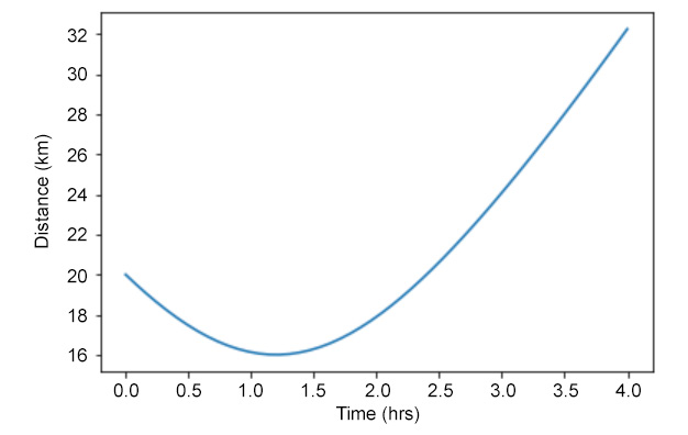
Figure 10.32: Plot of distance versus time
Note
To access the source code for this specific section, please refer to https://packt.live/38k2kuF.
You can also run this example online at https://packt.live/31FK3GG.
Activity 10.01: Maximum Circle-to-Cone Volume
This is a classic optimization problem, which results in some extremely complicated equations to differentiate and solve if you're doing it by hand. However, doing it with the help of Python will make the calculus part much easier. You start with a circle and cut out a sector of θ degrees. Then you attach points A and B in the following figure to make a cone:

Figure 10.33: Circle to cone volume
The problem, like in the box problem, is to find the angle to cut out which maximizes the volume of the cone. It will require you to visualize cutting out the angle, attach the points to make a cone, and calculate the volume of the resulting cone.
Steps for completion:
- Find the arc length of AB.
- Find h, the height of the resulting cone.
- Find r, the radius of the base of the cone.
- Find an expression for the volume of the cone as a function of theta (θ), the angle cut out.
Note
The solution to this activity can be found on page 694.
Summary
The tools of calculus allowed mathematicians and scientists to deal with constantly changing values, and those tools changed the way science is done. All of a sudden, we could use infinitely small steps to approximate the slope of a curve at a point, or infinitely small rectangles to approximate the area under a curve. These tools were developed hundreds of years before our modern world of computers and free programming software, but there's no reason to limit ourselves to the tools available to Newton, Leibniz, and the Bernoullis.
In this chapter, we learned to take derivatives of functions by simply dividing the rise of the function from one point to another by the infinitesimal run between those points. We simply told Python to divide 1 by a million to give us that small number. Without a computer, plugging those decimals into a function would be a daunting task, but Python plugs a decimal into a function as easily as a whole number.
We used the derivative idea to find the highest or lowest output of a function, where the derivative equals zero. This enabled us to find the optimal value of a function that would yield the shortest distance, or the greatest volume, for example.
The second most important topic in calculus is integration, and that allowed us to build up a complicated area or volume slice by slice using rectangles, trapezoids, or cylinders. Using Python, we could easily combine hundreds or thousands of slices to accurately approximate an area or volume.
We've only scratched the surface of the power that calculus and Python give us to work with changing values, infinitely small values, and infinitely large ones, too.
In the next chapter, we'll expand on these basic tools to find the lengths of curves, the areas of surfaces, and, most usefully for machine learning, the minimum point on a surface.
WFT54
GLS48