Overview
By the end of this chapter, you will be able to grasp the basic concepts of sequences and series and write Python functions that implement these concepts. You will understand the relationships between basic trigonometric functions and their applications, such as the famous Pythagorean theorem. You will practice vector calculus and know where it is applicable by performing vector algebra in Python. Finally, you will feel happy knowing that complex numbers are not any less a type of number; they are intimately connected to trigonometry and are useful for real-world applications.
Introduction
In the previous chapter, we covered functions and algebra with Python, starting with basic functions before working through transformations and solving equations. In this chapter, we'll introduce sequences and series, which have many applications in the real world, such as finance, and also form the basis for an understanding of calculus. Additionally, we will explore trigonometry, vectors, and complex numbers to give us a better understanding of the mathematical world.
The core skills of any exceptional Python programmer include a solid understanding of the background mathematics and an effective application of them. Think of vectors and complex numbers as valuable extensions to our mathematical toolbox that, later on, will contribute to efficiently describing, quantifying, and tackling real-world problems from the finance, science, or business and social domains.
Sequences and series, among others, appear in situations where profits, losses, dividends, or other payments occur on a regular basis. Trigonometry and trigonometric functions are necessary to solve geospatial problems, while vectors are applied widely in physics and engineering, machine learning, and more, where several different values are grouped together and the notion of direction is pivotal. Complex numbers are some of the most fundamental concepts that enjoy wide applications in electromagnetism, optics, quantum mechanics, and computer science.
Sequences and Series
If you were to participate in a TV show where the $10,000 question was "Given the numbers 2, 4, 8, 16, and 32, what comes next in the sequence?", what would your best guess be? If your response is 64, then congratulations—you just came closer to understanding one of the key concepts in mathematical abstraction: that of a sequence. A sequence is, pretty much like in the ordinary sense of the word, a particular order in which things follow each other. Here, things are (in most cases) integers or real numbers that are related. The order of the elements matters. The elements are also called the members or terms of the sequence.
For example, in the preceding sequence of the TV show you participated in, every term stems from the number prior being multiplied by 2; there is no end in this sequence as there is no end in the number of terms (integer numbers) you can come up with. In other instances, elements in a sequence can appear more than once. Think of the number of days in the months of a year, or just the sequence of the outcomes of a random event, say, the toss of a coin. A well-known sequence that has been known since the ancient Indian times is the Fibonacci sequence—1, 1, 2, 3, 5, 8, 13…. This is the sequence where each new term is the sum of the two previous terms.
That is, we need to know at least two terms before we can derive any other. In other words, we need to read the two first numbers (in the preceding sequence, 1 and 1, but generally any two numbers) before we are capable of deriving and predicting the third number. We know that some sequences, such as the Fibonacci sequence, include some logic inside them; a basic rule that we can follow and derive any term of the sequence.
In this chapter, we will be focusing on basic sequences, also known as progressions, that are repeatedly found across many fields in applied mathematics and programming that fall in either of the three basic categories: arithmetic, geometric, and recursive. These are not the only possibilities; they are, nonetheless, the most popular families of sequences and illustrate the logic that they entail.
A sequence of numbers {αn} = {α1, α2, α3, ..., αΝ, ...} is an ordered collection of terms (elements or members) for which there is a rule that associates each natural number n = 1, 2, 3, ..., N with just one of the terms in the sequence. The length of the sequence (that is, the number of its terms) can be finite or infinite, and the sequence is hence called finite or infinite, accordingly.
A series is a mathematical sequence that is summed as follows:
Figure 5.1: Equation of series
This can also be summed using the summation sign, as follows:

Figure 5.2: Equation of an infinite series
In the preceding case, our series is infinite (that is, it is the sum of all the terms of an infinite sequence). However, a series, such as a sequence, can also be finite. Why would a sum have infinite terms? Because it turns out that, in many cases, the summation is carried out computationally more efficiently by applying known formulas. Moreover, the summation can converge to a number (not infinite) or some function, even when the sequence is infinite. Due to this, series can be considered the building blocks of known functions, and their terms can be used to represent functions of increasing complexity, thus making the study of their properties intuitive. Series and sequences are ubiquitous in mathematics, physics, engineering, finance, and beyond and have been known since ancient times. They appear and are particularly useful as infinite sums in the definition of derivates and other functions as well.
Arithmetic Sequences
Like most mathematical concepts, sequences can be found everywhere in our daily lives. You might not have thought about it before, but every time you ride a cab, a sequence is running in the background to calculate the total cost of your ride. There is an initial charge that increments, by a fixed amount, for every kilometer (or mile) you ride. So, at any given moment, there's a real, corresponding number (the price of the ride so far). The ordered set of all these subtotals forms a sequence. Similarly, your body height as you grow up is a sequence of real numbers (your height expressed in centimeters or inches) in time (days or months). Both these examples constitute sequences that are non-decreasing in time—in other words, every term is either larger than or equal to any previous term, but never smaller. However, there is a subtle difference between the two examples: while the rate at which we gain height as we grow differs (growth is fast for kids, slow for teenagers, and zero for adults), the rate at which the taxi fare increases is constant. This leads us to need to introduce a special class of sequences—arithmetic sequences—which are defined as follows.
Sequences where the difference between any two consecutive terms is constant are called arithmetic. Hence, the formula for arithmetic sequences is as follows: αn+1- αn = d
Here, d is constant and must hold for all n. Of course, it becomes clear that, if you know the parameter d and some (any) term αn, then the term αn+1 can be found by a straightforward application of the preceding relation. By repetition, all the terms, αn+2, αn+3 ..., as well as the terms αn-1, αn-2 can be found. In other words, all of the terms of our sequence are known (that is, uniquely determined) if you know the parameter d, and the first term of the sequence α1. The general formula that gives us the nth term of the sequence becomes the following:
αn = α1 + (n – 1)d
Here, d is known as the common difference.
Inversely, to test whether a generic sequence is an arithmetic one, it suffices to check all of the pairwise differences, αn+1 – αn, of its terms and see whether these are the same constant number. In the corresponding arithmetic series, the sum of the preceding sequence becomes the following:
Σnj αj = Σnj [ α1 + (j – 1)d ] = n(α1 + αn)/2
This means that by knowing the length, n, the first, and the last term of the sequence, we can determine the sum of all terms from α1 to αn. Note that the sum (α1 + αn) gives twice the arithmetic mean of the whole sequence, so the series is nothing more than n times the arithmetic mean.
Now, we know what the main logic and constituents of the arithmetic sequence are. Now, let's look at some concrete examples. For now, we do not need to import any particular libraries in Python as we will be creating our own functions. Let's remind ourselves that these always need to begin with def, followed by a space, the function name (anything that we like), and a list of arguments that the function takes inside brackets, followed by a semi-colon. The following lines are indented (four places to the right) and are where the logic, that is, the algorithm or method of the function, is written. For instance, consider the following example:
def my_function(arg1, arg2):
'''Write a function that adds two numbers
and returns their sum'''
result = arg1 + arg2
return result
What follows the final statement, result, is what is being returned from the function. So, for instance, if we are programming the preceding my_function definition, which receives two input numbers, arg1 and arg2, then we can pass it to a new variable, say, the following one:
summed = my_function(2,9)
print(summed)
The output will be as follows:
11
Here, summed is a new variable that is exactly what is being returned (produced) by my_function. Note that if the return statement within the definition of a function is missing, then the syntax is still correct and the function can still be called. However, the summed variable will be equal to None.
Now, if we want to create a (any) sequence of numbers, we should include an iteration inside our function. This is achieved in Python with either a for or a while loop. Let's look at an example, where a function gives a sequence of n sums as the output:
def my_sequence(arg1, arg2, n):
'''Write a function that adds two numbers n times and
prints their sum'''
result = 0
for i in range(n):
result = result + arg1 + arg2
print(result)
Here, we initiate the variable result (to zero) and then iteratively add to it the sum, arg1 + arg2. This iteration happens n times, where n is also an argument of our new function, my_sequence. Every time the loop (what follows the for statement) is executed, the result increases by arg1 + arg2 and is then printed on-screen. We have omitted the return statement here for simplicity. Here, we used Python's built-in range() method, which generates a sequence of integer numbers that starts at 0 and ends at one number before the given stop integer (the number that we provide as input). Let's call our function:
my_sequence(2,9,4)
We will obtain the following output:
11
22
33
44
Had we used a while loop, we would have arrived at the same result:
def my_sequence(arg1, arg2, n):
'''Write a function that adds two numbers n times
and prints their sum'''
i = 0
result = 0
while i < n:
result = result + arg1 + arg2
print(result)
If we were to call the my_sequence function, we would obtain the same output that we received previously for the same input.
Generators
One more interesting option for sequential operations in Python is the use of generators. Generators are objects, similar to functions, that return an iterable set of items, one value at a time. Simply speaking, if a function contains at least one yield statement, it becomes a generator function. The benefit of using generators as opposed to functions is that we can call the generator as many times as desired (here, an infinite amount) without cramming our system's memory. In some situations, they can be invaluable tools. To obtain one term of a sequence of terms, we use the next() method. First, let's define our function:
def my_generator(arg1, arg2, n):
'''Write a generator function that adds
two numbers n times and prints their sum'''
i = 0
result = 0
while i < n:
result = result + arg1 + arg2
i += 1
yield result
Now, let's call the next() method multiple times:
my_gen = my_generator(2,9,4)
next(my_gen)
The following is the output:
11
Call the method for the second time:
next(my_gen)
The following is the output:
22
Call it for the third time:
next(my_gen)
The following is the output:
33
Call the method for the fourth time:
next(my_gen)
The following is the output:
44
So, we obtained the same results as in the previous example, but one at a time. If we call the next() method repetitively, we will get an error message since we have exhausted our generator:
next(my_gen)
Traceback (most recent call last):
File "<stdin>", line 1, in <module>
StopIteration
Now, we are ready to implement the relations of sequences we learned in Python code.
Exercise 5.01: Determining the nth Term of an Arithmetic Sequence and Arithmetic Series
In this exercise, we will create a finite and infinite arithmetic sequence using a simple Python function. As inputs, we want to provide the first term of the sequence, a1, the common difference, d, and the length of the sequence, n. Our goal is to obtain the following:
- Just one term (the nth term) of the sequence.
- The full sequence of numbers.
- The sum of n terms of the arithmetic sequence, in order to compare it to our result of the arithmetic series given previously.
To calculate the preceding goals, we need to provide the first term of the sequence, a1, the common difference, d, and the length of the sequence, n, as inputs. Let's implement this exercise:
- First, we want to write a function that returns just the nth term, according to the general formula αn = α1 + (n – 1)d:
def a_n(a1, d, n):
'''Return the n-th term of the arithmetic sequence.
:a1: first term of the sequence. Integer or real.
:n: the n-th term in sequence
returns: n-th term. Integer or real.'''
an = a1 + (n - 1)*d
return an
By doing this, we obtain the nth term of the sequence without needing to know any other preceding terms. For example, let's call our function with arguments (4, 3, 10):
a_n(4, 3, 10)
We will get the following output:
31
- Now, let's write a function that increments the initial term, a1, by d, n times and stores all terms in a list:
def a_seq(a1, d, n):
'''Obtain the whole arithmetic sequence up to n.
:a1: first term of the sequence. Integer or real.
:d: common difference of the sequence. Integer or real.
:n: length of sequence
returns: sequence as a list.'''
sequence = []
for _ in range(n):
sequence.append(a1)
a1 = a1 + d
return sequence
- To check the resulting list, add the following code:
a_seq(4, 3, 10)
The output will be as follows:
[4, 7, 10, 13, 16, 19, 22, 25, 28, 31]
Here, we obtained the arithmetic sequence, which has a length of 10, starts at 4, and increases by 3.
- Now, let's generate the infinite sequence. We can achieve this using Python generators, which we introduced earlier:
def infinite_a_sequence(a1, d):
while True:
yield a1
a1 = a1 + d
for i in infinite_a_sequence(4,3):
print(i, end=" ")
If you run the preceding code, you will notice that we have to abort the execution manually; otherwise, the for loop will print out the elements of the sequence eternally. An alternative way of using Python generators is, as explained previously, to call the next() method directly on the generator object (here, this is infinite_a_sequence()).
- Let's calculate the sum of the terms of our sequence by calling the sum() Python method:
sum(a_seq(4, 3, 10))
The output will be as follows:
175
- Finally, implement the αn = α1 + (n – 1)d formula, which gives us the arithmetic series so that we can compare it with our result for the sum:
def a_series(a1, d, n):
result = n * (a1 + a_n(a1, d, n)) / 2
return result
- Run the function, as follows:
a_series(4, 3, 10)
The output is as follows:
175.0
Note
To access the source code for this specific section, please refer to https://packt.live/2D2S52c.
You can also run this example online at https://packt.live/31DjRfO.
With that, we have arrived at the same result for the summation of elements of an arithmetic sequence by using either a sequence or series. The ability to cross-validate a given result with two independent mathematical methods is extremely useful for programmers at all levels and lies at the heart of scientific validation. Moreover, knowing different methods (here, the two methods that we used to arrive at the series result) that can solve the same problem, and the advantages (as well as the disadvantages) of each method can be vital for writing code at an advanced level.
We will study a different, but also fundamental, category of sequences: geometric ones.
Geometric Sequences
An infectious disease spreads from one person to another or more, depending on the density of the population in a given community. In a situation such as a pandemic, for a moderately contagious disease, it is realistic that, on average, each person who has the disease infects two people per day. So, if on day 1 there is just one person that's infected, on day 2 there will be two newly infected, and on day 3, another two people will have contracted the disease for each of the two previously infected people, bringing the number of the newly infected to four. Similarly, on day 4, eight new cases appear, and so on. We can see that the rate that a disease expands at is not constant since the number of new cases depends on the number of existing cases at a given moment—and this explains how pandemics arise and spread exponentially.
The preceding numbers (1, 2, 4, 8...) form a sequence. Note that now, the requirement of the arithmetic sequence hasn't been met: the difference between two successive terms is not constant. The ratio, nonetheless, is constant. This exemplifies the preceding sequence as a special type of sequence, known as geometric, and is defined as a sequence or a collection of ordered numbers where the ratio of any two successive terms is constant.
In the compact language of mathematics, we can write the preceding behavior as αn+1 = r αn.
Here, αn is the number of cases on day n, αn+1 is the number of new cases on day n+1, and r>0 is a coefficient that defines how fast (or slow) the increase happens. This is known as the common ratio. The preceding formula is universal, meaning that it holds for all members, n. So, if it holds true for n, it does so for n-1, n-2, and so on. By working with the preceding relationship recursively, we can easily arrive at αn = rn-1α equation.
Here, we give the nth term of the geometric sequence once the first term, α=α1, and the common ratio, r, have been given. The term α is known as the scale factor.
Note that r can have any non-zero value. If r>1, every generation, αn+1, is larger than the one prior and so the sequence is ever-increasing, while the opposite is true if r<1: αn+1 tends towards zero as n increases. So, in the initial example of an infectious disease, r>1 means that the transmission is increasing, while r<1 yields a decreasing transmission.
Let's write a Python function that calculates the nth term of a geometric function, based on the αn = rn-1α formula:
def n_geom_seq(r, a, n):
an = r**(n-1) * a
return an
The inputs in that function are r, the common ratio, a, the scale factor, and n, the nth term that we want to find. Let's call this function with some arguments, (2, 3, 10):
n_geom_seq(2, 3, 10)
The output is as follows:
1536
Similarly, for the case of the arithmetic sequence, we define a geometric series as the sum of the terms of the sequence of length n:

Figure 5.3: A geometric sequence
Alternatively, we can express this as follows:

Figure 5.4: Alternative expression for a geometric sequence
To get a better understanding of the geometric series, let's check out how it works in Python and visualize it. We need to define a function that admits r, a, and n (as we did previously) as input and calculate the second formula, that is, the series up to term n:
def sum_n(r, a, n):
sum_n = a*(1 - r**n) / (1 - r)
return sum_n
Now, call the function for arguments (2, 3, 10), as we did previously:
sum_n(2, 3, 10)
The output is as follows:
3069.0
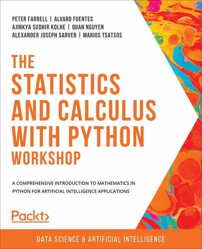
Have a look at the following example plot of geometric sequences, where the value increases for r>1:
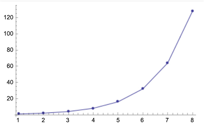
Figure 5.5: Geometric sequences increasing for r>1
Have a look at the following example plot of geometric sequences, where the value decreases for r<1:
Figure 5.6: Geometric sequences decreasing for r<1
In this section, we have seen how a geometric sequence progresses and how we can easily find the terms of it in Python, as well as the geometric series. We are now ready to implement what we've learned in an exercise in order to obtain a better understanding of sequences and their applications.
Exercise 5.02: Writing a Function to Find the Next Term of the Sequence
The number of bacteria in a Petri dish increases as a geometric sequence. Given the population (number) of bacteria per day, across a number of days, n, write a function that calculates the population on day n+1. Follow these steps to complete this exercise:
- Write a function that admits a variable number of arguments (*args) and calculates the ratio between any element and its preceding element (starting from the second element). Then, check whether all the ratios found are identical and return their unique value. Otherwise, the function returns -1 (the sequence does not possess a unique common ratio):
def find_ratio(*args):
arg0=args[0]
ratios = []
for arg in args[1:]:
ratio = round(arg/arg0,8)
arg0=arg
ratios.append(ratio)
if len(set(ratios)) == 1:
return ratio
else:
return -1
- Now, check the find_ratio function for two distinct cases. First, let's use the following sequence:
find_ratio(1,2,4,8,16,32,64,128,256,512)
The output is as follows:
2.0
- Now, let's use the following sequence:
find_ratio(1,2,3)
The output is as follows:
-1
As shown in the preceding outputs, the find_ratio function prints out the ratio, if it exists, or prints -1 if the sequence is not geometric.
- Now, write a second function that reads in a sequence and prints out what the next term will be. To do so, read in a (comma-separated) list of numbers, find their ratio, and from that, predict the next term:
def find_next(*args):
if find_ratio(*args) == -1:
raise ValueError('The sequence you entered'
'is not a geometric sequence. '
'Please check input.')
else:
return args[-1]*find_ratio(*args)
Note that we want to check whether the sequence possesses a common ratio by calling the find_ratio() function we wrote previously. If it doesn't, raise an error; if it does, find the next term and return it.
- Check if it works by using the following sequence:
find_next(1,2,4)
The following is the output of the preceding code:
8.0
- Now, try this with a different sequence:
find_next(1.36,0.85680,0.539784,0.34006392)
The output is as follows:
0.2142402696
It does work. In the first case, the obvious result, 8.0, was printed. In the second case, the less obvious result of the decreasing geometric sequence was found and printed out. To summarize, we are able to write a function that detects a geometric sequence, finds its ratio, and uses that to predict the next-in-sequence term. This is extremely useful in real-life scenarios, such as in cases where the compound interest rate needs to be verified.
Note
To access the source code for this specific section, please refer to https://packt.live/2NUyT8N.
You can also run this example online at https://packt.live/3dRMwQV.
In the previous sections, we saw that sequences, either arithmetic or geometric, can be defined in two equivalent ways. We saw that the nth term of the sequence is determined by knowing a given term of the sequence (commonly the first, but not necessarily) and the common difference, or common ratio. More interestingly, we saw that the nth term of a sequence can be found by knowing the (n-1)th term, which, in turn, can be found by knowing the (n-2)th term, and so on. So, there is an interesting pattern here that dictates both sequence types that we studied and which, in fact, extends beyond them. It turns out that we can generalize this behavior and define sequences in a purely recursive manner that isn't necessarily arithmetic or geometric. Now, let's move on to the next section, where we will understand recursive sequences.
Recursive Sequences
A recursive sequence is a sequence of elements, υn, that are produced via a recursive relation, that is, each element uniquely stems from the preceding ones.
υn can depend on one or more elements preceding it. For example, the Fibonacci series that we saw earlier in this chapter is a recursive sequence where knowledge of the nth term requires knowing both the (n-1)th and (n-2)th terms. On the other hand, the factorial only needs the element that precedes it. Specifically, it is defined by the recurrence relation, n! = n(n-1)! , n > 0, and the initial condition, 0! = 1.
Let's convert the preceding formulas into Python code:
def factorial(n):
if n == 0 or n ==1:
return 1
elif n == 2:
return 2
else:
return n*factorial(n - 1)
The preceding code is a recursive implementation of the factorial function: to calculate the result for n, we call the function for n-1, which, in turn, calls the function for n-2 and so on until n=2 is reached.
If we execute the preceding function for the case n=11, we obtain the following:
factorial(11)
The output is as follows:
39916800
Note that while the first two categories of sequences that we've seen so far (arithmetic and geometric) are mutually exclusive, the recursive family of sequences is not, meaning that sequences can be both recursive and arithmetic or recursive and geometric. Conventionally, we use the term recursive for these types of sequences that, unlike geometric and arithmetic, cannot be expressed in a non-recursive manner.
Now that we have explored the basic concepts of recursive sequences, we can implement this in Python and write code that calculates any number of elements of any sequence that is recursively defined.
Exercise 5.03: Creating a Custom Recursive Sequence
In this exercise, we will create a custom recursive sequence using the concepts we explained in the previous section. Given the first three elements of the sequence, Pn, that is, P1=1, P2=7, and P3=2, find the next seven terms of the sequence that is recursively defined via the relation: Pn+3= (3*Pn+1 - Pn+2)/(Pn – 1). Follow these steps to complete this exercise:
- Define a Python function that is recursive and implements the relation given previously for the nth element of the sequence:
def p_n(n):
if n < 1:
return -1
elif n == 1:
return 1
elif n == 2:
return 7
elif n == 3:
return 2
else:
pn = (3*p_n(n-2) - p_n(n-1) )/ (p_n(n-3) + 1)
return pn
Here, we started by defining the base cases, that is, the known result as given in the brief: if n=1, then P=1, if n=2, then P=7, and if n=3, then P=2. We also included the case where n<1. This is invalid input and, as is customary, our function returns the value -1. This makes our function bounded and protected from entering infinite loops and invalid input. Once these cases have been taken care of, then we have defined the recursive relation.
- Now, let's test our function and print out the first 10 values of the sequence (three that correspond to the base cases and seven of them that are for our task):
for i in range(1,11):
print(p_n(i))
The output is as follows:
1
7
2
9.5
-0.4375
9.645833333333334
-1.0436507936507937
53.29982363315697
-5.30073825572847
-3784.586609737289
As you can see from the preceding output, our function works and gives back both the known values (P1 = 1, P2 = 7, and P3 = 2) of the sequence and the next terms (P_1 to P_10) that we were looking for.
- As a bonus, let's plot our findings by using the matplotlib module. We will create a list that holds the first nine values of the sequence and then plot it with pyplot:
from matplotlib import pyplot as plt
plist = []
for i in range(1,40):
plist.append(p_n(i))
plt.plot(plist, linestyle='--', marker='o', color='b')
plt.show()
The output is as follows:

Figure 5.7: Plot created using the matplotlib library
Note
To access the source code for this specific section, please refer to https://packt.live/2D3vlPF.
You can also run this example online at https://packt.live/3eY05Q4.
We can see that a simple and well-defined recursive relation can lead to apparently random or chaotic results. Indeed, if you continue plotting the terms of the preceding sequence, you will soon notice that there is no apparent regularity in the pattern of the terms as they widely and asymmetrically oscillate around 0. This prompts us to arrive at the conclusion that even though defining a recursive sequence and predicting its nth term is straightforward, the opposite is not always true. As we saw, given a sequence (a list of numbers), it is quite simple to check whether it forms an arithmetic sequence, a geometric sequence, or neither. However, to answer whether a given sequence has been derived by a recursive relation—let alone what this recursion is—is a non-trivial task that, in most cases, cannot be answered.
In this section, we have presented what sequences are, why they are important, and how they are connected to another important concept in mathematics: series. We studied three general types of sequences, namely arithmetic, geometric, and recursive, and saw how they can be implemented in Python in a few simple steps. In the next section, we'll delve into trigonometry and learn how trigonometric problems can be easily solved using Python.
Trigonometry
Trigonometry is about studying triangles and, in particular, the relation of their angles to their edges. The ratio of two of the three edges (sides) of a triangle gives information about a particular angle, and to such a pair of sides, we give it a certain name and call it a function. The beauty of trigonometry and mathematics in general is that these functions, which are born inside a triangle, make (abstract) sense in any other situation where triangles are not present and operate as independent mathematical objects. Hence, functions such as the tangent, cosine, and sine are found across most fields of mathematics, physics, and engineering without any reference to the triangle.
Let's look at the most fundamental trigonometric functions and their usage.
Basic Trigonometric Functions
We will start by defining a right-angled triangle (or simply a right triangle), triangle ABC. One of its angles (the angle BCA in the following diagram) is a right angle, that is, a 90-degree angle. The side opposite the right angle is called the hypotenuse (side h in the following diagram), while the other sides (a and b) are known as legs. They are also referred to as opposite and adjacent to the respective angle. For instance, side b is adjacent to the lower right angle in the following diagram (angle CAB or θ), while it is opposite when we refer to the top angle (angle CBA):
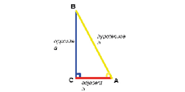
Figure 5.8: A right-angled triangle
The most common trigonometric functions are defined with the help of the preceding diagram and are defined as follows:

Figure 5.9: Trigonometric functions
For the tangent function, it also holds that tanθ = sinθ/cosθ.
Also, for any angle, θ, the following identity always holds true: sinθ2 + cosθ2 = 1.
By construction, the trigonometric functions are periodic. This means that, regardless of the sizes of the edges of a triangle, the preceding functions take on values that repeat themselves every 2π. This will become apparent in the next exercise, where we will be plotting them. The range of the sine and cosine functions is the interval [-1,1]. This means that the smallest value they can obtain is -1, and the largest is 1, no matter what the input θ is.
Last but not least, the edges of the right-angled triangle are connected via the famous Pythagorean theorem: h2 = a2 + b2
In Python code, a simple implementation of the Pythagorean theorem would be to write a function that calculates h, given a and b, with the help of the square root (sqrt) method of the math module; for instance:
from math import sqrt
def hypotenuse(a,b):
h = sqrt(a**2 + b**2)
return h
Calling this function for a=3 and b=4 gives us the following:
hypotenuse(a = 3, b = 4)
The output is as follows:
5.0
Now, let's look at some concrete examples so that we can grasp these ideas.
Exercise 5.04: Plotting a Right-Angled Triangle
In this exercise, we will write Python functions that will plot a right triangle for the given points, p1 and p2. The right-angled triangle will correspond to the endpoints of the legs of the triangle. We will also calculate the three trigonometric functions for either of the non-right angles. Let's plot the basic trigonometry functions:
- Import the numpy and pyplot libraries:
import numpy as np
from matplotlib import pyplot as plt
Now, write a function that returns the hypotenuse by using the Pythagorean theorem when given the two sides, p1 and p2, as inputs:
def find_hypotenuse(p1, p2):
p3 = round( (p1**2 + p2**2)**0.5, 8)
return p3
- Now, let's write another function that implements the relations for the sin, cos, and tan functions. The inputs are the lengths of the adjacent, opposite, and hypotenuse of a given angle, and the result is a tuple of the trigonometric values:
def find_trig(adjacent, opposite, hypotenuse):
'''Returns the tuple (sin, cos, tan)'''
return opposite/hypotenuse, adjacent/hypotenuse,
opposite/adjacent
- Now, write the function that plots the triangle. For simplicity, place the right angle at the origin of the axes at (0,0), the first input point along the x axis at (p1, 0), and the second input point along the y axis at (0, p2):
def plot_triangle(p1, p2, lw=5):
x = [0, p1, 0]
y = [0, 0, p2]
n = ['0', 'p1', 'p2']
fig, ax = plt.subplots(figsize=(p1,p2))
# plot points
ax.scatter(x, y, s=400, c="#8C4799", alpha=0.4)
ax.annotate(find_hypotenuse(p1,p2),(p1/2,p2/2))
# plot edges
ax.plot([0, p1], [0, 0], lw=lw, color='r')
ax.plot([0, 0], [0, p2], lw=lw, color='b')
ax.plot([0, p1], [p2, 0], lw=lw, color='y')
for i, txt in enumerate(n):
ax.annotate(txt, (x[i], y[i]), va='center')
Here, we created the lists, x and y, that hold the points and one more list, n, for the labels. Then, we created a pyplot object that plots the points first, and then the edges. The last two lines are used to annotate our plot; that is, add the labels (from the list, n) next to our points.
- We need to choose two points in order to define a triangle. Then, we need to call our functions to display the plot:
p01 = 4
p02 = 4
print(find_trig(p01,p02,find_hypotenuse(p01,p02)))
plot_triangle(p01,p02)
The first line prints the values of the three trigonometric functions, sin, cos, and tan, respectively. Then, we plot our triangle, which in this case is isosceles since it has two sides that are of equal length.
The output will be as follows:

Figure 5.10: Plotting the isosceles triangle
The results are expected and correct—upon rounding the error—since the geometry of this particular shape is simple (an isosceles orthogonal triangle that has two angles equal to π/4). Then, we checked the result (note that in NumPy, the value of pi can be directly called np.pi).
- Finally, to get a general overview of the sin and cos trigonometric functions, let's plot them:
x = np.linspace(0, 10, 200)
sin = np.sin(x)
cos = np.cos(x)
plt.xticks([0, np.pi/2, np.pi, 3*np.pi/2, 2*np.pi,
5*np.pi/2, 3*np.pi],
['0','','u03C0','','2u03C0','','3u03C0'])
plt.plot(x, sin, marker='o', label='sin')
plt.plot(x, cos, marker='x', label='cos')
plt.legend(loc="upper left")
plt.ylim(-1.1, 1.6)
plt.show()
The output will be as follows:
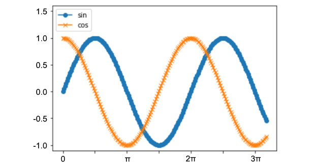
Figure 5.11: Plot of the sin and cos trigonometric functions
In this exercise, we kick-started our explorations of the sphere of trigonometry and saw how to arrive at useful visualizations in Python.
Note
To access the source code for this specific section, please refer to https://packt.live/2Zz0TnU.
You can also run this example online at https://packt.live/2AoxS63.
With that, we have established the main trigonometric functions and saw how these provide an operation between an angle and an associated trigonometric value, given by either the sin, cos, or tan function. Moreover, we saw that these three functions are periodic, that is, repeated every 2π, while the first two are bounded, that is, the values they can take never exceed the interval, [-1,1]. These values are directly found in Python or in a scientific pocket calculator. In many situations, however, the inverse process is desired: can I find the angle if I give the value of sin, cos, or tan to some function? Does such a function exist? We'll answer these questions in the next section.
Inverse Trigonometric Functions
Inverse trigonometric functions are the inverse functions of the trigonometric functions and are just as useful as their counterparts. An inverse function is a function that reverses the operation or result of the original function. Recall that trigonometric functions admit angles as input values and output pure numbers (ratios). Inverse trigonometric functions do the opposite: they admit a pure number as input and give an angle as output. So, if, for instance, a point, π, is mapped to point -1 (as the cos function does), then its inverse needs to do exactly the opposite. This mapping needs to hold for every point where the inverse function is defined.
The inverse function of the sin(x) function is called arcsin(x): if y=sin(x), then x=arcsin(y). Recall that sin is a periodic function, so many different x's are mapped to the same y. So, the inverse function would map one point to several different ones. This cannot be allowed since it clashes with the very definition of a function. To avoid this drawback, we need to restrict our domain of arcsin (and similarly for arccos) to the interval [-1,1], while the images, y=arcsin(x) and y=arccos(x), are restricted to the ranges [-π/2,π/2] and [0, π] respectively.
We can define the three basic inverse trigonometric functions as follows:
- arcsin(x) = y such that arcsin(sin(x)) = x
- arccos(x) = y such that arccos(cos(x)) = x
- arctan(x) = y such that arctan(tan(x)) = x
In Python, these functions can be called either from the math module or from within the numpy library. Since most Python implementations of trigonometric inverse functions return radians, we may want to convert the outcome into degrees. We can do this by multiplying the radians by 180 and then dividing by π.
Let's see how this can be written in code. Note that the input, x, is expressed as a pure number between -1 and 1, while the output is expressed in radians. Let's import the required libraries and declare the value of x:
from math import acos, asin, atan, cos
x = 0.5
Now, to print the inverse of cosine, add the following code:
print(acos(x))
The output is as follows:
1.0471975511965979
To print the inverse of sine, add the following code:
print(asin(x))
The output is as follows:
0.5235987755982989
To print the inverse of tan, add the following code:
print(atan(x))
The output is as follows:
0.4636476090008061
Let's try adding an input to the acos function that's outside the range [-1,1]:
x = -1.2
print(acos(x))
We will get an error, as follows:
Traceback (most recent call last):
File "<stdin>", line 1, in <module>
Something similar will happen for asin. This is to be expected since no angle, φ, exists that can return -1.2 as cos (or sin). However, this input is permitted in the atan function:
x = -1.2
print(atan(x))
The output is as follows:
-0.8760580505981934
Last, let's check what the inverse of the inverse arccos(cos(x)) function gives us:
print(acos(cos(0.2)))
The output is as follows:
0.2
As expected, we retrieve the value of the input of the cos function.
The inverse trigonometric functions have a variety of applications across mathematics, physics, and engineering. For example, calculating integrals can be done by using inverse trigonometric functions. The indefinite integrals are as follows:
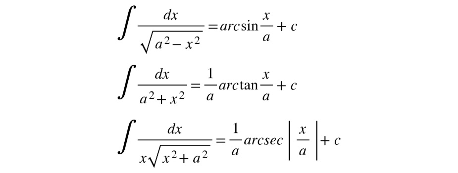
Figure 5.12: Inverse trigonometric functions
Here, a is a parameter and C is a constant, and the integrals become immediately solvable with the help of inverse trigonometric functions.
Exercise 5.05: Finding the Shortest Way to the Treasure Using Inverse Trigonometric Functions
In this exercise, you will be given a secret map that points to B, where some precious treasure has been lying for centuries. You are at point A and the instructions are clear: you have to navigate 20 km south then 33 km west so that you arrive at the treasure. However, the straight-line segment, AB, is the shortest. You need to find the angle θ on the map so that your navigation is correctly oriented:

Figure 5.13: Graphical representation of the points A, B, and C
We need to find the angle θ, which is the angle between the segments AB and AC. Follow these steps:
- Import the atan (arctan or inverse tangent) function:
from math import atan, pi
- Find the tangent of θ using BC and AC:
AC = 33
BC = 20
tan_th = BC/AC
print(tan_th)
The output is as follows:
0.6060606060606061
- Next, find the angle by taking the inverse tangent function. Its argument is the tangent of θ:
theta = atan(tan_th)
- Convert that into degrees and print the value:
theta_degrees = theta*180/pi
print(theta_degrees)
The output is as follows:
31.218402764346372
So, the answer is that we need to turn 31.22 degrees in order to navigate correctly.
- As a bonus point, calculate the distance that we will travel along the path AB. This is simply given by the Pythagorean theorem as follows:
AB2 = AC2 + BC2
In Python, use the following code:
AB = (AC**2 + BC**2)**0.5
print(AB)
The output is as follows:
38.58756276314948
The course will be 38.59 km.
It is straightforward to calculate this in Python by calling the find_hypotenuse() function. As expected, this is much shorter than the path AC + BC = 53 km.
Note
To access the source code for this specific section, please refer to https://packt.live/31CF4qr.
You can also run this example online at https://packt.live/38jfVlI.
Exercise 5.06: Finding the Optimal Distance from an Object
You are visiting your local arena to watch your favorite show, and you are standing in the middle of the arena. Besides the main stage, there is also a viewing screen so that people can watch and not miss the details of the show. The bottom of the screen stands 3 m above your eye level, and the screen itself is 7 m high. The angle of vision is formed by looking at both the bottom and top of the screen. Find the optimal distance, x, between yourself and the screen so that the angle of vision is maximized:

Figure 5.14: Angle of vision formed between the eyes and the screen
This is a slightly involved problem that requires a bit of algebra, but we will break it down into simple steps and explain the logic. First, note how much the plot of the problem guides us and helps us arrive at a solution. This apparently complex real-world problem translates into a much more abstract and simple geometric picture. Follow these steps to complete this exercise:
- Calculate x. This is the lower side of the triangle and also the adjacent side to the angle, θ1 (and also θ=θ1+θ2). The answer, x, will be given by the condition that the viewing angle, θ2 or equivalently, tan(θ2)), is maximized. From the preceding plot of the screen, we can immediately draw the following relations for the three angles: θ1 (the inner angle), θ2 (the outer angle), and θ=θ1+θ2:
tan(θ1) = opposite/adjacent = 3/x
tan(θ) = tan(θ1+θ2) = opposite/adjacent = (7+3)/x .
Now, use algebra to work around these two relations and obtain a condition for θ2.
- A known identity for the tangent of a sum of two angles is as follows:

Figure 5.15: Formula for tangent of a sum of two angles
By substituting what we have found for tan(θ) and tan(θ1) in the latter relation and after working out the algebra, we arrive at the following:
tan(θ2) = 7x/(30+x2) or
θ2 = arctan(7x/(30+x2)).
In other words, we have combined the elements of the problem and found that the angle, θ1, ought to change with the distance, x, as a function of x, which was given in the preceding line.
- Let's plot this function to see how it changes. First, load the necessary libraries:
from matplotlib import pyplot as plt
import numpy as np
- Then, plot the function by defining the domain, x, and the values, y, by using the arctan method of numpy. These are easily plotted with the plot() method of pyplot, as follows:
x = np.linspace(0.1, 50, 2000)
y = np.arctan(7*x / (30+x**2) )
plt.plot(x,y)
plt.show()
The output will be as follows:
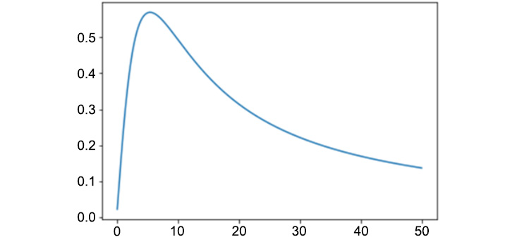
Figure 5.16: Plot of the function using the arctan method
From the preceding graph, we can see that the functions obtain a maximum.
- Determine the function's maximum value, y, and the position, x, where this occurs:
ymax = max(y)
xmax = x[list(y).index(ymax)]
print(round(xmax,2), round(ymax,2))
The output is as follows:
5.47 0.57
- Lastly, convert the found angle into degrees:
ymax_degrees = round(ymax * 180 / np.pi, 2)
print(ymax_degrees)
The output is as follows:
32.58
So, the viewing angle, θ2, is at its maximum at 32.58 degrees and occurs when we stand 5.47 m away from the screen. We used the trigonometric and inverse trigonometric functions, implemented them in Python, and found the answer to a problem that arises from a geometric setup in a real-life situation. This sheds more light on how concepts from geometry and trigonometry can be usefully and easily coded to provide the expected results.
Note
To access the source code for this specific section, please refer to https://packt.live/2VB3Oez.
You can also run this example online at https://packt.live/2VG9x2T.
Now, we will move on and study another central concept in mathematics with a wide range of applications in algebra, physics, computer science, and applied data science: vectors.
Vectors
Vectors are abstract mathematical objects with a magnitude (size) and direction (orientation). A vector is represented by an arrow that has a base (tail) and a head. The head shows the direction of the vector, while the length of the arrow's body shows its magnitude.
A scalar, in contrast to a vector, is a sole number. It's a non-vector, that is, a pure integer, real or complex (as we shall see later), that has no elements and hence no direction.
Vectors are symbolized by either a bold-faced letter A, a letter with an arrow on top, or simply by a regular letter, if there is no ambiguity regarding the notation in the discussion. The magnitude of the vector, A, is stylized as |A| or simply A. Now, let's have a look at the various vector operations.
Vector Operations
Simply put, a vector is a collection (think of a list or array) of two, three, or more numbers that form a mathematical object. This object lives in a particular geometrical space called a vector space that has some properties, such as metric properties, and dimensionality. A vector space can be two-dimensional (think of the plane of a sheet of your book), three-dimensional (the ordinary Euclidean space around us), or higher, in many abstract situations in mathematics and physics. The elements or numbers that are needed to identify a vector equals the dimensionality of the space. Now that we have defined a vector space—the playground for vectors—we can equip it with a system of axes (the usual x, y, and z axes) that mark the origin and measure the space. In such a well-defined space, we need to determine a set of numbers (two, three, or more) in order to uniquely define a vector, since vectors are assumed to begin at the origin of axes. The elements of a vector can be integers, rational, real, or (rarely) complex numbers. In Python, they are, most commonly, represented by lists or NumPy arrays.
Similar to real numbers, a set of linear operations is defined on vectors. Between two vectors, A = (a1, a2, a3) and B = (b1, b2, b3), we can define the following:
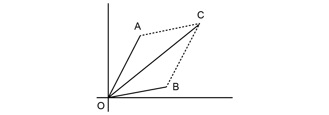
Figure 5.17: Points A, B, and C and their relations while performing vector operations
Now let us see the various operations that can be performed on these vectors:
- Addition as the operation that results in vector C = A + B = (a1 + b1, a2 + b2, a3 + b3).
- Subtraction as the operation that results in vector C = A - B = (a1 - b1, a2 - b2, a3 - b3).
- Dot (or inner or scalar) product of the scalar C = b. b = a1 b1 + a2 b2 + a3 b3.
- Cross (or exterior) product of the vector C = A x B, which is perpendicular to the plane define by A and B and has elements (a2b3 - a3b2, a3b1 - a1b3, a1b2 – a2b1).
- Element-wise or Hadamard product of two vectors, A and B, is the vector, C, whose elements are the pairwise product of elements of A and B; that is, C = (a1 b1, a2 b2, a3 b3).
We can define and use the preceding formulas in Python code as follows:
import numpy as np
A = np.array([1,2,3]) # create vector A
B = np.array([4,5,6]) # create vector B
Then, to find the sum of A and B, enter the following code:
A + B
The output is as follows:
array([5, 7, 9])
To calculate the difference, enter the following code:
A - B
The output is as follows:
array([-3, -3, -3])
To find the element-wise product, enter the following code:
A*B
The output is as follows:
array([ 4, 10, 18])
To find the dot product, use the following code:
A.dot(B)
The output is as follows:
32
Finally, the cross product can be calculated as follows:
np.cross(A,B)
The output is as follows:
array([-3, 6, -3])
Note that vector addition, subtraction, and the dot product are associative and commutative operations, whereas the cross product is associative but not commutative. In other words, a x b does not equal b x a, but rather b x a, which is why it is called anticommutative.
Also, a vector, A, can be multiplied by a scalar, λ. In that case, you simply have to multiply each vector element by the same number, that is, the scalar: λ A = λ (a1, a2, a3) = (λ a1, λ a2, λ a3)
Another important operation between vectors is the dot product, since it is arguably the most common operation to appear in mathematics, computer science, and its applications. The dot product is a funny type of operation that has no analog in the realm of real numbers. Indeed, it needs two vectors as input to produce a single scalar as output. This means that the result of the operation (scalar) is of a different type than its ingredients (vectors), and thus an inverse operation (a dot division) cannot generally exist.
By definition, it is given as follows:
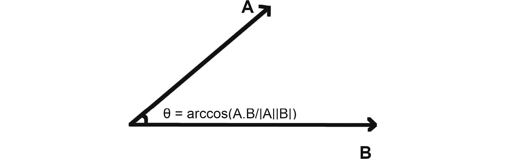
Figure 5.18: Graphical representation of the θ angle
This can be represented by the following equation:
A.B = |A| |B| cos(θ)
Here, θ is the angle between A and B.
Let's have a look at some typical cases:
- If A and B are orthogonal, then the dot product vanishes:
A.B = 0 if and only if θ = angle(A,B) = π/2, since |A| and |B| are not zero.
- If A and B are co-linear and co-directional, then θ = 0, cos(θ)=1 and A.B = |A| |B|. If they are co-linear and have opposite directions, then θ = π, cos(θ)=-1, and A.B = -|A| |B|.
- It follows on from the definition for the dot product of a vector with itself: A.A = |A| |A| or |A| = √(A.A)
- It follows directly from A.B = |A| |B| cos(θ), where the angle between the two vectors is given as follows: θ = arccos(A.B / |A| |B|)
Here, arccos is the inverse cos function that we saw in the previous section.
For example, we can write a Python program that calculates the angle between any two given vectors with the help of numpy and the preceding relation that gives us the angle, θ:
import numpy as np
from math import acos
A = np.array([2,10,0])
B = np.array([9,1,-1])
To find the norm (magnitude) of each vector, we can use the following code:
Amagn = np.sqrt(A.dot(A))
Bmagn = np.sqrt(B.dot(B))
As an alternative, you can also use the following code:
Amagn = np.linalg.norm(A)
Bmagn = np.linalg.norm(B)
Print their values:
print(Amagn, Bmagn)
You will get the following output:
10.198039027185569
9.1104335791443
Both alternatives lead to the same result, which you can immediately check by printing Amagn and Bmagn once more.
Finally, we can find the angle, θ, as follows:
theta = acos(A.dot(B) / (Amagn * Bmagn))
print(theta)
The output is as follows:
1.2646655256233297
Now, let's have a look at exercise where will perform the various vector operations that we just learned about.
Exercise 5.07: Visualizing Vectors
In this exercise, we will write a function that plots two vectors in a 2D space. We'll have to find their sum and the angle between them.
Perform the following steps to complete this exercise:
- Import the necessary libraries, that is, numpy and matplotlib:
import numpy as np
import matplotlib.pyplot as plt
- Create a function that admits two vectors as inputs, each as a list, plots them, and, optionally, plots their sum vector:
def plot_vectors(vec1, vec2, isSum = False):
label1 = "A"; label2 = "B"; label3 = "A+B"
orig = [0.0, 0.0] # position of origin of axes
The vec1 and vec2 lists hold two real numbers each. Each pair denotes the endpoint (head) coordinates of the corresponding vector, while the origin is set at (0,0). The labels are set to "A", "B", and "A+B", but you could change them or even set them as variables of the plot_vectors function with (or without) default values. The Boolean variable, isSum, is, by default, set to False and the sum, vec1+vec2, will not be plotted unless it's explicitly set to True.
- Next, we put the coordinates on a matplotlib.pyplot object:
ax = plt.axes()
ax.annotate(label1, [vec1[0]+0.5,vec1[1]+0.5] )
# shift position of label for better visibility
ax.annotate(label2, [vec2[0]+0.5,vec2[1]+0.5] )
if isSum:
vec3 = [vec1[0]+vec2[0], vec1[1]+vec2[1]]
# if isSum=True calculate the sum of the two vectors
ax.annotate(label3, [vec3[0]+0.5,vec3[1]+0.5] )
ax.arrow(*orig, *vec1, head_width=0.4, head_length=0.65)
ax.arrow(*orig, *vec2, head_width=0.4, head_length=0.65,
ec='blue')
if isSum:
ax.arrow(*orig, *vec3, head_width=0.2,
head_length=0.25, ec='yellow')
# plot the vector sum as well
plt.grid()
e=3
# shift limits by e for better visibility
plt.xlim(min(vec1[0],vec2[0],0)-e, max(vec1[0],
vec2[0],0)+e)
# set plot limits to the min/max of coordinates
plt.ylim(min(vec1[1],vec2[1],0)-e, max(vec1[1],
vec2[1],0)+e)
# so that all vectors are inside the plot area
Here, we used the annotate method to add labels to our vectors, as well as the arrow method, in order to create our vectors. The star operator, *, is used to unpack the arguments within the list's orig and vec1, vec2 so that they are read correctly from the arrow() method. plt.grid() creates a grid on the plot's background to guide the eye and is optional. The e parameter is added so that the plot limits are wide enough and the plot is readable.
- Next, we give our graph a title and plot it:
plt.title('Vector sum',fontsize=14)
plt.show()
plt.close()
- Now, we will write a function that calculates the angle between the two input vectors, as explained previously, with the help of the dot (inner) product:
def find_angle(vec1, vec2, isRadians = True, isSum = False):
vec1 = np.array(vec1)
vec2 = np.array(vec2)
product12 = np.dot(vec1,vec2)
cos_theta = product12/(np.dot(vec1,vec1)**0.5 *
np.dot(vec2,vec2)**0.5 )
cos_theta = round(cos_theta, 12)
theta = np.arccos(cos_theta)
plot_vectors(vec1, vec2, isSum=isSum)
if isRadians:
return theta
else:
return 180*theta/np.pi
First, we map our input lists to numpy arrays so that we can use the methods of this module. We calculate the dot product (named product12) and then divide that by the product of the magnitude of vec1 with the magnitude of vec2. Recall that the magnitude of a vector is given by the square root (or **0.5) of the dot product with itself. As given by the definition of the dot product, we know that this quantity is the cos of the angle theta between the two vectors. Lastly, after rounding cos to avoid input errors in the next line, calculate theta by making use of the arccos method of numpy.
- We want to combine the two functions that we wrote—find_angle and plot_vectors—and call the former inside the latter. We also want to give the user the option to print the result for the angle either in radians (isRadians=True) or degrees (isRadians=False). We are now ready to try our function. First, let's try this with two perpendicular vectors:
ve1 = [1,5]
ve2 = [5,-1]
find_angle(ve1, ve2, isRadians = False, isSum = True)
The output is as follows:
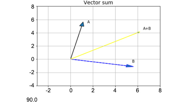
Figure 5.19: Plot of two perpendicular vectors
The plot looks good and the result is 90 degrees, as expected.
- Now, let's try using the same function to create two co-linear vectors:
ve1 = [1,5]
ve2 = [0.5,2.5]
find_angle(ve1, ve2, isRadians = False, isSum = True)
The output is as follows:

Figure 5.20: Plot of two co-linear vectors
The output is 0 degrees, as expected.
- Lastly, again, using the same function, let's create two generic vectors:
ve1 = [1,5]
ve2 = [-3,-5]
find_angle(ve1, ve2, isRadians = False, isSum = True)
The output is as follows:

Figure 5.21: Plot of two generic vectors
In summary, we have studied vectors as mathematical objects that live in a vector space. We have learned how to construct and represent vectors in Python and how to visualize them. Vectors follow some simple rules, and performing operations with them is possible. Addition and subtraction follow exactly the same logic when dealing with real numbers. Multiplication is somewhat more involved and different types of products are defined. The most common product is the inner or dot product, which enjoys wide popularity in the mathematical and physics communities due to its simple geometric representation. We learned how to calculate the dot product of any two vectors in Python and, moreover, found the angle between the duet by using our knowledge (and some NumPy methods) of the dot product. In simple terms, a vector, in two dimensions, is a pair of numbers that form a geometric object with interesting properties.
Note
To access the source code for this specific section, please refer to https://packt.live/2Zxu7n5.
You can also run this example online at https://packt.live/2YPntJQ.
Next, we will learn how a pair of two numbers can be combined into an even more exciting object, that of a complex number.
Complex Numbers
Mathematical ideas have been evolving regarding numbers and their relationships since ancient numerical systems. Historically, mathematical ideas have evolved from concrete to abstract ones. For instance, a set of natural numbers was created so that all physical objects in the world around us directly correspond to some number within this set. Since arithmetic and algebra have developed, it has become clear that numbers beyond the naturals or integers are necessary, so decimal and rational numbers were introduced. Similarly, around the times of Pythagoras, it was found that rational numbers cannot solve all numerical problems that we could construct with the geometry that was known at that time. This happened when irrational numbers—numbers that result from taking the square root of other numbers and that have no representation as ratios—were introduced.
Complex numbers are an extension of real numbers and include some special numbers that can provide a solution to some equations that real numbers cannot.
Such a number does, in fact, exist and has the symbol i. It is called an imaginary number or imaginary unit, even though there is nothing imaginary about it; it is as real as all the other numbers that we have seen and has, as we shall see, some very beautiful properties.
Basic Definitions of Complex Numbers
We define the imaginary number i as follows:
i2 = -1
Any number that consists of a real and an imaginary number (part) is called a complex number. For example, consider the following numbers:
z = 3 – i
z = 14/11 + i 3
z = -√5 – i 2.1
All the preceding numbers are all complex numbers. Their real part is symbolized as Re(z) and their imaginary part is symbolized as Im(z). For the preceding examples, we get the following:
Re(z) = 3 , Im(z) = -1
Re(z) = 14/11 , Im(z) = 3
Re(z) = -√5 , Im(z) = -2.1
Let's look at some examples using code. In Python, the imaginary unit is symbolized with the letter j and a complex number is written as follows:
c = <real> + <imag>*1j,
Here, <real> and <imag> are real numbers. Equivalently, a complex number can be defined as follows:
c = complex(<real>, <imag>).
In code, it becomes as follows:
a = 1
b = -3
z = complex(a, b)
print(z)
The output is as follows:
(1-3j)
We can also use the real and imag functions to separate the real and imaginary parts of any complex number, z. First, let's use the real function:
print(z.real)
The output is as follows:
1.0
Now, use the imag function:
print(z.imag)
The output is as follows:
-3.0
In other words, any complex number can be decomposed and written as z=Re(z) + i Im(z). As such, a complex number is a pair of two real numbers and can be visualized as a vector that lives in two dimensions. Hence, the geometry and algebra of vectors, as discussed in the previous section, can be applied here as well.
Methods and functions that admit complex numbers as inputs are found in the cmath module. This module contains mathematical functions for complex numbers. The functions there accept integers, floating-point numbers, or complex numbers as input arguments.
A complex conjugate is defined as the complex number, z* (also z̄), that has the same real part as the complex number, z, and the opposite imaginary part; that is, if z = x+iy, then z* = x -iy. Note that the product, zz*, is the real number, x2+y2, which gives us the square of the modulus of z:
zz* = z*z = |z|2
A complex number is plotted, similar to a vector, on the complex plane (as shown in the following diagram). This is the plane that's formed by the real part on the x axis and the imaginary part on the y axis. The complex conjugate is simply a reflection of the vector with respect to the real axis:
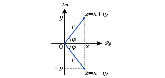
Figure 5.22: A plot of a complex number
A complex number, z, can be visualized as a vector with coordinates (x, y). Alternatively, we can write it as a vector with polar coordinates (r, φ). The complex conjugate, z* or z̄, is a vector the same as z but reflected with respect to the x axis.
A complex number is zero if both its real and complex parts are zero. The following operations can be performed on two complex numbers, z = x+iy and w = u+iv:
- Addition: z+w = (x+u) + i(y+v)
- Subtraction: z-w = (x-u) + i(y-v)
- Multiplication: z w = (x+iy)(u+iv) = (xu-yv) + i(xv + yu)
- Division: z/w = (x+iy)/(u+iv) = (ux+vy)+i(uy-xv) / (u2+v2)
Polar Representation and Euler's Formula
A complex number is easily visualized as a vector on the complex plane. As such, it has a magnitude, which is determined by the vector's size, and an orientation, which is determined by the angle, φ, that is formed with the x (real) axis. To determine these two numbers, we need to find the absolute value (or modulus), r, of z=x+iy:
r = |z| = √x2+y2
Its angle (also, called the argument, arg, or phase), φ, is as follows:
φ = arg(z) = arctan(x+iy) = arctan(y/x)
Both of these relations stem from the geometry of the complex vector. The first relation is simply the application of the Pythagorean theorem, while the second comes from applying the tangent relation to the angle, φ.
By examining the graphical representation of the vector (see the preceding diagram), we can see the following:
cos(φ) = x/r and
sin(φ) = y/r
Or
x = r cos(φ) and
y = r sin(φ)
By substituting these with z = x+iy, we get the following:
z = r (cos(φ) + i sin(φ))
We can write some code in Python to find (r, φ) (the polar coordinates) once (x, y) (the cartesian coordinates) are given and vice versa:
def find_polar(z):
from math import asin
x = z.real
y = z.imag
r = (x**2 + y**2)**0.5
phi = asin(y/r)
return r, phi
find_polar(1-3j)
The output is as follows:
(3.1622776601683795, -1.2490457723982544)
Equivalently, we can use the polar method from the cmath module:
import cmath
z = 1-3j
cmath.polar(z)
The output is as follows:
(3.1622776601683795, -1.2490457723982544)
Note
The input (0,0) is not allowed since it leads to division by zero.
Therefore, a complex number can be represented by its modulus, r, and phase, φ, instead of its abscissa (x, the real part) and ordinate (y, the imaginary part). The modulus, r, is a real, non-negative number and the phase, φ, lies in the interval [-π,π]: it is 0 and π for purely real numbers and π/2 or -π/2 for purely imaginary numbers. The latter representation is called polar, while the former is known as rectangular or Cartesian; they are equivalent. The following representation is also possible:
z = r eiφ = r (cos(φ) + i sin(φ))
Here is the base of the natural logarithm. This is known as Euler's formula. The special case, φ=π, gives us the following:
eiπ + 1 = 0
This is known as Euler's identity.
The benefit of using Euler's formula is that complex number multiplication and division obtain a simple geometric representation. To multiply (divide) two complex numbers, z1 and z2, we simply multiply (divide) their respective moduli and add (subtract) their arguments:
z1 * z2 = r eiφ = r1 * r2 ei(φ1+φ2)
Now, let's implement some mathematical operations with complex numbers in Python. We will code the addition, subtraction, multiplication, and division of two complex numbers:
def complex_operations2(c1, c2):
print('Addition =', c1 + c2)
print('Subtraction =', c1 - c2)
print('Multiplication =', c1 * c2)
print('Division =', c1 / c2)
Now, let's try these functions for a generic pair of complex numbers, c1=10+2j/3 and c2=2.9+1j/3:
complex_operations2(10+2j/3, 2.9+1j/3)
The output is as follows:
Addition = (12.9+1j)
Subtraction = (7.1+0.3333333333333333j)
Multiplication = (28.77777777777778+5.266666666666666j)
Division = (3.429391054896336-0.16429782240187768j)
We can do the same for a purely real number with a purely imaginary number:
complex_operations2(1, 1j)
The output is as follows:
Addition = (1+1j)
Subtraction = (1-1j)
Multiplication = 1j
Division = -1j
From the last line, we can easily see that 1/i = -i, which is consistent with the definition of the imaginary unit. The cmath library also provides useful functions for complex numbers, such as phase and polar, as well as trigonometric functions for complex arguments:
import cmath
def complex_operations1(c):
modulus = abs(c)
phase = cmath.phase(c)
polar = cmath.polar(c)
print('Modulus =', modulus)
print('Phase =', phase)
print('Polar Coordinates =', polar)
print('Conjugate =',c.conjugate())
print('Rectangular Coordinates =',
cmath.rect(modulus, phase))
complex_operations1(3+4j)
The output is as follows:
Modulus = 5.0
Phase = 0.9272952180016122
Polar Coordinates = (5.0, 0.9272952180016122)
Conjugate = (3-4j)
Rectangular Coordinates = (3.0000000000000004+3.9999999999999996j)
Hence, calculating the modulus, phase, or conjugate of a given complex number becomes extremely simple. Note that the last line gives us back the rectangular (or Cartesian) form of a complex number, given its modulus and phase.
Now that we learned how the arithmetic and representation of complex numbers work, let's move on and look at an exercise that involves logic and combines what we have used and learned about in the previous sections.
Exercise 5.08: Conditional Multiplication of Complex Numbers
In this exercise, you will write a function that reads a complex number, c, and multiplies it by itself if the argument of the complex number is larger than zero, takes the square root of c if its argument is less than zero, and does nothing if the argument equals zero. Plot and discuss your findings:
- Import the necessary libraries and, optionally, suppress any warnings (this isn't necessary but is helpful if you wish to keep the output tidy from warnings that depend on the versions of the libraries you're using):
import cmath
from matplotlib import pyplot as plt
import warnings
warnings.filterwarnings("ignore")
- Now, define a function that uses Matplotlib's pyplot function to plot the vector of the input complex number, c:
def plot_complex(c, color='b', label=None):
ax = plt.axes()
ax.arrow(0, 0, c.real, c.imag, head_width=0.2,
head_length=0.3, color=color)
ax.annotate(label, xy=(0.6*c.real, 1.15*c.imag))
plt.xlim(-3,3)
plt.ylim(-3,3)
plt.grid(b=True, which='major') #<-- plot grid lines
- Now, create a function that reads the input complex number, c, plots it by calling the function defined previously, and then investigates the different cases, depending on the phase of the input. Plot the phases before and after the operation, as well as the result, in order to compare the resulting vector with the input vector:
def mult_complex(c, label1='old', label2='new'):
phase = cmath.phase(c)
plot_complex(c, label=label1)
if phase == 0:
result = -1
elif phase < 0:
print('old phase:', phase)
result = cmath.sqrt(c)
print('new phase:', cmath.phase(result))
plot_complex(result, 'red', label=label2)
elif phase > 0:
print('old phase:', phase)
result = c*c
print('new phase:', cmath.phase(result))
plot_complex(result, 'red', label=label2)
return result
Note that for negative phases, we take the square root of c (using the math.sqrt() method), whereas for positive phases, we take the square of c.
- Now, transform a number that lies on the upper half of the complex plane:
mult_complex(1 + 1.2j)
The output is as follows:
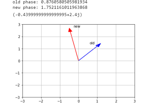
Figure 5.23: The plot of a number that lies on the upper half of the complex plane
Here, a complex number with a positive argument, φ (blue vector), is being transformed (or mapped) to a new complex number (red vector) with a larger modulus and a new argument that is twice the previous value. This is expected: remember Euler's formula for the polar representation of c=r eiφ? It becomes obvious that the square, c2, is a number with double the original argument, φ, and modulus, r2.
- Next, transform a number that lies on the lower half of the complex plane:
mult_complex(1-1.2j)
The output is as follows:

Figure 5.24: Plot of a number that lies on the lower half of the complex plane
In this case, the square root is calculated. Similar to the first example, the newly transformed vector has a modulus that is the square root of the modulus of the original vector and an argument that is half of the original one.
Note
Fun fact: In both cases, the vector has been rotated anti-clockwise.
- Write a while iteration that calls the mult_complex() function n times to check what happens if we keep the vectors rotating:
c0 = 1+1.2j
n = 0
while n < 6:
c0 = mult_complex(c0, None, str(n))
n+=1
The output is as follows:
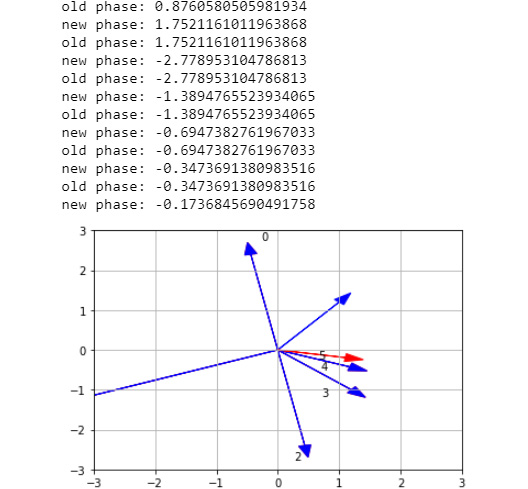
Figure 5.25: Plot of rotating vectors
With that, we've seen how vectors and vector algebra can be used to visualize geometric operations. In particular, dividing and multiplying complex numbers results in acquiring a geometric representation that can be helpful when dealing with large sets of data and visualizations.
Note
To access the source code for this specific section, please refer to https://packt.live/31yU8W1.
You can also run this example online at https://packt.live/2BXWJOw.
Activity 5.01: Calculating Your Retirement Plan Using Series
In many countries, a retirement plan (also known as 401(k)) is offered by some employers. Such plans allow you to contribute directly from your paycheck, so they are an easy and effective way to save and invest for retirement. You have been tasked with writing some code that calculates and plots your monthly return based on the amount and duration of contributions.
A retirement plan accumulates in time, exactly like a geometric series does. It is an investment: you save money on a monthly basis in order to collect it later, on a monthly basis, with added value or interest. The main ingredients to calculate the retirement return are your current balance, a monthly contribution, the employer match (employer's contribution), the retirement age, the rate of return (the average annual return you expect from your 401(k) investment), life expectancy, and any other fees. In a realistic case, caps are introduced: the employer match (typically between 50% and 100%) cannot be raised by more than 6% of your annual salary. Similarly, the employee's contribution cannot be larger than a given amount in a year (typically, this is 18 K), regardless of how high the salary is.
Perform the following steps to complete this activity:
- Identify the variables of our problem. These will be the variables of our functions. Make sure you read through the activity description carefully and internalize what is known and what is to be calculated.
- Identify the sequence and write one function that calculates the value of the retirement plan at some year, n. The function should admit the current balance, annual salary, year, n, and more as inputs and return a tuple of contribution, employer's match, and total retirement value at year n.
- Identify the series and write one function that calculates the accumulated value of the retirement plan after n years. The present function should read the input, call the previous function that calculates the value of the plan at each year, and sum all the (per year) savings. For visualization purposes, the contributions (per year), employer match (per year), and total value (per year) should be returned as lists in a tuple.
- Run the function for a variety of chosen values and ensure it runs properly.
- Plot the results with Matplotlib.
Note
The solution for this activity can be found on page 672.
Summary
In this chapter, you have been provided with a general and helpful exposition of the most central mathematical concepts in sequences, series, trigonometry, vectors, and complex numbers and, more importantly, their implementation in Python using concrete and short examples. As a real-life example, we examined a retirement plan and the progression of our savings in time. However, numerous other situations can be modeled after sequences or series and be studied by applying vectors or complex numbers. These concepts and methods are widely used in physics, engineering, data science, and more. Linear algebra, that is, the study of vectors, matrices, and tensors, heavily relies on understanding the concept of geometry and vectors and appears almost everywhere in data science and when studying neural networks. Geometry and trigonometry, on the other hand, are explicitly used to model physical motion (in video games, for instance) and more advanced concepts in geospatial applications. However, having background knowledge of these concepts makes using and applying data science methods more concrete and understandable.
In the next chapter, we will discuss matrices and how to apply them to solve real-world problems. We'll also examine Markov chains, which are used to tie concepts regarding probability, matrices, and limits together.
NDN74
ETB65