By the end of this chapter, you will be familiar with basic and foundational concepts in probability theory. You'll learn how to use NumPy and SciPy modules to perform simulations and solve problems by calculating probabilities using simulations. This chapter also covers how to calculate the probabilities of events using simulations and theoretical probability distributions. Along with this, we'll conceptually define and use random variables included in the scipy.stats module. We will also understand the main characteristics of the normal distribution and calculate probabilities by computing the area under the curve of the probability distribution.
Introduction
In the previous chapter, we learned how to perform the first steps in any statistical analysis. Given a business or scientific problem and a related dataset, we learned how to load the dataset and prepare it for analysis. Then, we learned how to calculate and use descriptive statistics to make sense of the variables. Finally, we performed EDA to complement the information we gathered from the descriptive statistics and gained a better understanding of the variables and their possible relationships. After getting a basic understanding of an analytical problem, you may need to go one step further and use more sophisticated quantitative tools, some of which are used in the following fields:
- Inferential statistics
- Machine learning
- Prescriptive analytics
- Optimization
What do all of these domains have in common? Many things: for example, they have a mathematical nature, they make heavy use of computational tools, and in one way or another they use probability theory, which is one of the most useful branches of applied mathematics and provides the foundation and tools for other disciplines, such as the ones mentioned previously.
In this chapter, we'll give a very brief introduction to probability theory. Unlike traditional statistical books, in this chapter, we'll make heavy use of simulations to put the theoretical concepts into practice and make them more concrete. For this, we will make extensive use of NumPy's and SciPy's random number generation capabilities and we will learn how to use simulations to solve problems. After introducing the mandatory foundational concepts, we'll show you how to produce random numbers using NumPy and use these capabilities to calculate probabilities. After doing that, we'll define the concept of random variables.
Later in this chapter, we'll delve deeper into the two types of random variables: discrete and continuous, and for each type, we will learn how to create random variables with SciPy, as well as how to calculate exact probabilities with these distributions.
Randomness, Probability, and Random Variables
This is a dense section, with many theoretical concepts to learn. Although it is heavy, you will finish this section with a very good grasp of some of the most basic and foundational concepts in probability theory. We will also introduce very useful methods you can use to perform simulations using NumPy so that you get to play around with some code. By using simulations, we hope to show you how the theoretical concepts translate into actual numbers and problems that can be solved with these tools. Finally, we will define random variables and probability distribution, two of the most important concepts to know about when using statistics to solve problems in the real world.
Randomness and Probability
We all have an intuitive idea of the concept of randomness and use the term in everyday life. Randomness means that certain events happen unpredictably or without a pattern.
One paradoxical fact about random events is that although individual random events are, by definition, unpredictable, when considering many such events, it is possible to predict certain results with very high confidence. For instance, when flipping a coin once, we cannot know which of the two possible outcomes we will see (heads or tails). On the other hand, when flipping a coin 1,000 times, we can be almost sure that we will get between 450 and 550 heads.
How do we go from individually unpredictable events to being able to predict something meaningful about a collection of them? The key is probability theory, the branch of mathematics that formalizes the study of randomness and the calculation of the likelihood of certain outcomes. Probability can be understood as a measure of uncertainty, and probability theory gives us the mathematical tools to understand and analyze uncertain events. That's why probability theory is so useful as a decision-making tool: by rigorously and logically analyzing uncertain events, we can reach better decisions, despite the uncertainty.
Uncertainty can come from either ignorance or pure randomness, in such a way that flipping a coin is not a truly random process if you know the mass of the coin, the exact position of your fingers, the exact force applied when throwing it, the exact gravitational pull, and so on. With this information, you could, in principle, predict the outcome, but in practice, we don't know all these variables or the equations to actually make an exact prediction. Another example could be the outcome of a football (soccer) game, the results of a presidential election, or if it's going to rain one week from now.
Given our ignorance about what will happen in the future, assigning a probability is what we can do to come up with a best guess.
Probability theory is also a big business. Entire industries, such as lotteries, gambling, and insurance, have been built around the laws of probability and how to monetize the predictions we can make from them. The casino does not know if the person playing roulette will win in the next game, but because of probability laws, the casino owner is completely sure that roulette is a profitable game. The insurance company does not know if a customer will have a car crash tomorrow, but they're sure that having enough car insurance costumers paying their premiums is a profitable business.
Although the following section will feel a bit theoretical, it is necessary to get to know the most important concepts before we can use them to solve analytical problems.
Foundational Probability Concepts
We will start with the basic terminology that you will find on most treatments of this subject. We must learn these concepts in order to be able to solve problems rigorously and to communicate our results in a technically correct fashion.
We will start with the notion of an experiment: a situation that happens under controlled conditions and from which we get an observation. The result we observe is called the outcome of the experiment. The following table presents some examples of experiments, along with some possible outcomes:

Figure 8.1: Example experiments and outcomes
The sample space of the experiment consists of the mathematical set of all possible outcomes. Finally, an event is any subset of the sample space. Each element of the sample space is called a simple event because it consists of a single element. We now have four terms that are related to each other and that are essential to probability theory: experiment, sample space, event, and outcome. To continue with our examples from the previous table, the following table presents the sample space and examples of events for the experiments:
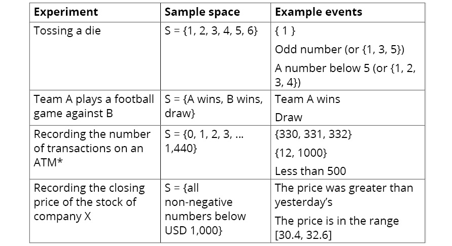
Figure 8.2: Example experiments, sample spaces, and events
Note
Please note that the details in the preceding table are assuming a maximum of 1 transaction per minute is happening.
It is worth noting that we defined the sample space as a set in the mathematical sense. Therefore, we can use all the mathematical operations we know from set theory, including getting subsets (which are events). As events are subsets of a larger set, they are sets themselves, and we can use unions, intersections, and so on. The conventional notation for events is to use uppercase letters such as A, B, and C.
We say that an event has happened when the outcome of the experiment belongs to the event. For example, in the experiment tossing a die, if we are interested in the event getting an odd number and we observe any of the outcomes, that is, 1, 3, or 5, then we can say that the event has happened.
When performing a random experiment, we don't know which outcome we are going to get. What we do in probability theory is assign a number to all the possible events related to an experiment. This number is what we know as the probability of an event.
How do we assign probabilities to events? There are a couple of alternatives. However, regardless of the method we use to assign probabilities to events, the theory of probability and its results hold if our way of assigning probabilities to events fulfills the following four conditions. Given events A and B and their probabilities, denoted as P(A) and P(B):
 : The probability of an event is always a number between 0 and 1. The closer to 1, the more likely the event will occur. The extremes are 0 for an event that can't occur and 1 for an event that will certainly occur.
 : If A is the empty set, then the probability must be 0. For instance, for the experiment tossing a die, the event getting a number greater than 10 does not exist, hence this is the empty set and its probability is 0.
 : This basically says that when performing an experiment, some outcome must occur for sure.
 for disjoint events A and B: If we have a collection of non-overlapping events, A and B, then the probability the event (A U B), also known as A or B, can be obtained by adding the individual probabilities. These rules also apply for more than two events.
This subsection has been heavy in terms of concepts and theory, but it is important to understand these now, in order to avoid mistakes later. Fortunately, we have Python and NumPy with their great numerical capabilities that will help us put this theory into practice.
Note
A quick note on all the exercises and related test scripts: If you are using a CLI (such as Windows' Command Prompt or Mac's Terminal) to run the test scripts, it will throw an error, such as Implement enable_gui in a subclass. This is something to do with some of the commands being used in the notebooks (such as %matplotlib inline). So, if you want to run the test scripts, please use the IPython shell. The code for the exercises in this book is best run on Jupyter Notebooks.
Introduction to Simulations with NumPy
To start putting all this theory into practice, let's begin by loading the libraries we will use in this chapter:
import pandas as pd
import numpy as np
import matplotlib.pyplot as plt
import seaborn as sns
# line to allow the plots to be shown in the Jupyter Notebook
%matplotlib inline
We will make extensive use of NumPy's random number generation capabilities. We will use the random module (np.random), which is able to generate random numbers that follow many of the most important probability distributions (more on probability distributions later).
Let's begin by simulating a random experiment: tossing a regular die.
Let's learn how to perform this experiment using NumPy. There are different ways to do this. We'll use the function randint from the random module, which generates random integers between low (inclusive) and high (exclusive) arguments. Since we want to generate numbers between 1 and 6, our function will look like this:
def toss_die():
outcome = np.random.randint(1, 7)
return outcome
Let's use our function ten times in a row to observe how it works:
for x in range(10):
print(toss_die())
The following is an example output:
6, 2, 6, 5, 1, 3, 3, 6, 6, 5
Since these numbers are randomly generated, you will most likely get different values.
For this function and almost every other function that produces random numbers (or some other random result), it is sometimes necessary to generate random numbers in such a way that anyone running the code at any moment obtains the same results. For that, we need to use a seed.
Let's add a line that creates the seed and then use our function ten times in a row to observe how it works:
np.random.seed(123)
for x in range(10):
print(toss_die(), end=', ')
The result is as follows:
6, 3, 5, 3, 2, 4, 3, 4, 2, 2
As long as you run the first line containing the number 123 inside the seed function, anyone running this code (with the same NumPy version) will get the same output numbers.
Another useful function from the numpy.random module is np.random.choice, which can sample elements from a vector. Say we have a class of 30 students, and we would like to randomly chose four of them. First, we generate the fictional student list:
students = ['student_' + str(i) for i in range(1,31)]
Now, can use np.random.choice to randomly select four of them:
sample_students = np.random.choice(a=students, size=4,
replace=False)
sample_students
The following is the output:
array(['student_16', 'student_11', 'student_19',
'student_26'], dtype='<U10')
The replace=False argument ensures that once an element has been chosen, it can't be selected again. This is called sampling without replacement.
In contrast, sampling with replacement means that all the elements of the vector are considered when producing each sample. Imagine that all the elements of the vector are in a bag. We randomly pick one element for each sample and then put the element we got in the bag before drawing the next sample. An application of this could be as follows: say that we will give a surprise quiz to one student of the group, every week for 12 weeks. All the students are subjects who may be given the quiz, even if that student was selected in a previous week. For this, we could use replace=True, like so:
sample_students2 = np.random.choice(a=students,
size=12, replace=True)
for i, s in enumerate(sample_students2):
print(f'Week {i+1}: {s}')
The result is as follows:
Week 1: student_6
Week 2: student_23
Week 3: student_4
Week 4: student_26
Week 5: student_5
Week 6: student_30
Week 7: student_23
Week 8: student_30
Week 9: student_11
Week 10: student_6
Week 11: student_13
Week 12: student_5
As you can see, poor student 6 was chosen on weeks 1 and 10, and student 30 on 6 and 8.
Now that we know how to use NumPy to generate dice outcomes and get samples (with or without replacement), we can use it to practice probability.
Exercise 8.01: Sampling with and without Replacement
In this exercise, we will use random.choice to produce random samples with and without replacement. Follow these steps to complete this exercise:
- Import the NumPy library:
import numpy as np
- Create two lists containing four different suits and 13 different ranks in the set of standard cards:
suits = ['hearts', 'diamonds', 'spades', 'clubs']
ranks = ['Ace', '2', '3', '4', '5', '6', '7', '8',
'9', '10', 'Jack', 'Queen', 'King']
- Create a list, named cards, containing the 52 cards of the standard deck:
cards = [rank + '-' + suit for rank in ranks for suit in suits]
- Use the np.random.choice function to draw a hand (five cards) from the deck. Use replace=False so that each card gets selected only once:
print(np.random.choice(cards, size=5, replace=False))
The result should look something like this (you might get different cards):
['Ace-clubs' '5-clubs' '7-clubs' '9-clubs' '6-clubs']
- Now, create a function named deal_hands that returns two lists, each with five cards drawn from the same deck. Use replace=False in the np.random.choice function. This function will perform sampling without replacement:
def deal_hands():
drawn_cards = np.random.choice(cards, size=10,
replace=False)
hand_1 = drawn_cards[:5].tolist()
hand_2 = drawn_cards[5:].tolist()
return hand_1, hand_2
To print the output, run the function like so:
deal_hands()
You should get something like this:
(['9-spades', 'Ace-clubs', 'Queen-diamonds', '2-diamonds',
'9-diamonds'],
['Jack-hearts', '8-clubs', '10-clubs', '4-spades',
'Queen-hearts'])
- Create a second function called deal_hands2 that's identical to the last one, but with the replace=True argument in the np.random.choice function. This function will perform sampling with replacement:
def deal_hands2():
drawn_cards = np.random.choice(cards, size=10,
replace=True)
hand_1 = drawn_cards[:5].tolist()
hand_2 = drawn_cards[5:].tolist()
return hand_1, hand_2
- Finally, run the following code:
np.random.seed(2)
deal_hands2()
The result is as follows:
(['Jack-hearts', '4-clubs', 'Queen-diamonds', '3-hearts',
'6-spades'],
['Jack-clubs', '5-spades', '3-clubs', 'Jack-hearts', '2-clubs'])
As you can see, by allowing sampling with replacement, the Jack-hearts card was drawn in both hands, meaning that when each card was sampled, all 52 were considered.
In this exercise, we practiced the concept of sampling with and without replacement and learned how to apply it using the np.random.choice function.
Note
To access the source code for this specific section, please refer to https://packt.live/2Zs7RuY.
You can also run this example online at https://packt.live/2Bm7A4Y.
Probability as a Relative Frequency
Let's return to the question of the conceptual section: how do we assign probabilities to events? Under the relative frequency approach, what we do is repeat an experiment a large number of times and then define the probability of an event as the relative frequency it has occurred, that is, how many times we observed the event happening, divided by the number of times we performed the experiment:

Figure 8.3: Formula to calculate the probability
Let's look into this concept with a practical example. First, we will perform the experiment of tossing a die 1 million times:
np.random.seed(81)
one_million_tosses = np.random.randint(low=1,
high=7, size=int(1e6))
We can get the first 10 values from the array:
one_million_tosses[:10]
This look like this:
array([4, 2, 1, 4, 4, 4, 2, 2, 6, 3])
Remember that the sample space of this experiment is S = {1, 2, 3, 4, 5, 6}. Let's define some events and assign them probabilities using the relative frequency method. First, let's use a couple of simple events:
- A: Observing the number 2
- B: Observing the number 6
We can use the vectorization capabilities of NumPy and count the number of simple events happening by summing the Boolean vector we get from performing the comparison operation:
N_A_occurs = (one_million_tosses == 2).sum()
Prob_A = N_A_occurs/one_million_tosses.shape[0]
print(f'P(A)={Prob_A}')
The result is as follows:
P(A)=0.16595
Following the exact same procedure, we can calculate the probability for event B:
N_B_occurs = (one_million_tosses == 6).sum()
Prob_B = N_B_occurs/one_million_tosses.shape[0]
print(f'P(B)={Prob_B}')
The result is as follows:
P(B)=0.166809
Now, we will try with a couple of compounded events (they have more than one possible outcome):
- C: Observing an odd number (or {1, 3, 5})
- D: Observing a number less than 5 (or {1, 2, 3, 4})
Because the event observing an odd number will occur if we get a 1 or 3 or 5, we can translate the or that we use in our spoken language into the mathematical OR operator. In Python, this is the | operator:
N_odd_number = (
(one_million_tosses == 1) |
(one_million_tosses == 3) |
(one_million_tosses == 5)).sum()
Prob_C = N_odd_number/one_million_tosses.shape[0]
print(f'P(C)={Prob_C}')
The result is as follows:
P(C)=0.501162
Finally, let's calculate the probability of D:
N_D_occurs = (one_million_tosses < 5).sum()
Prob_D = N_D_occurs/one_million_tosses.shape[0]
print(f'P(D)={Prob_D}')
We get the following value:
Here, we have used the relative frequency approach to calculate the probability of the following events:
- A: Observing the number 2: 0.16595
- B: Observing the number 6: 0.166809
- C: Observing an odd number: 0.501162
- D: Observing a number less than 5: 0.666004
In summary, under the relative frequency approach, when we have a set of outcomes from repeated experiments, what we do to calculate the probability of an event is count how many times the event has happened and divide that count by the total number of experiments. As simple as that.
In other cases, the assignments of probabilities can arise based on a definition. This is what we may call theoretical probability. For instance, a fair coin, by definition, has an equal probability of showing either of the two outcomes, say, heads or tails. Since there are only two outcomes for this experiment {heads, tails} and the probabilities must add up to 1, each simple event must have a 0.5 probability of occurring.
Another example is as follows: a fair die is one where the six numbers have the same probability of occurring, so the probability of tossing any number must be equal to 1/6 = 0.1666666. In fact, the default behavior of the numpy.randint function is to simulate the chosen integer numbers, each with the same probability of coming out.
Using the theoretical definition, and knowing that we have simulated a fair die with NumPy, we can arrive at the probabilities for the events we presented previously:
- A: Observing the number 2, P(A) = 1/6 = 0.1666666
- B: Observing the number 6, P(B) = 1/6 = 0.1666666
- C: Observing an odd number: P(observing 1 or observing 3 or observing 5) = P(observing 1) + or P(observing 3) + P(observing 5) = 1/6 + 1/6 + 1/6 = 3/6 = 0.5
- D: Observing a number less than 5: P(observing 1 or observing 2 or observing 3 or observing 4) = P(observing 1) + or P(observing 2) + P(observing 3) + P(observing 4) = 1/6 + 1/6 + 1/6 + 1/6 = 4/6 = 0.666666
Notice two things here:
- These numbers are surprisingly (or unsurprisingly, if you already knew this) close to the results we obtained by using the relative frequency approach.
- We could decompose the sum of C and D because of rule 4 of the Foundational Probability Concepts section.
Defining Random Variables
Often, you will find quantities whose values are (or seem to be) the result of a random process. Here are some examples:
- The sum of the outcome of two dice
- The number of heads when throwing ten coins
- The price of the stock of IBM one week from now
- The number of visitors to a website
- The number of calories ingested in a day by a person
All of these are examples of quantities that can vary, which means they are variables. In addition, since the value they take depends partially or entirely on randomness, we call them random variables: quantities whose values are determined by a random process. The typical notation for random variables is uppercase letters at the end of the alphabet, such as X, Y, and Z. The corresponding lowercase letter is used to refer to the values they take. For instance, if X is the sum of the outcomes of two dice, here are some examples of how to read the notation:
- P(X = 10): Probability of X taking the number 10
- P(X > 5): Probability of X taking a value greater than 5
- P(X = x): Probability of X taking the value x (when we are making a general statement)
Since X is the sum of two numbers from two dice, X can take the following values: {2, 3, 4, 5, 6, 7, 8, 9, 10, 11, 12}. Using what we learned in the previous section, we can simulate a large number of values for our random variable, X, like this:
np.random.seed(55)
number_of_tosses = int(1e5)
die_1 = np.random.randint(1,7, size=number_of_tosses)
die_2 = np.random.randint(1,7, size=number_of_tosses)
X = die_1 + die_2
We have simulated 100,000 die tosses for two dice and got the respective values for X. These are the first values for our vectors:
print(die_1[:10])
print(die_2[:10])
print(X[:10])
The result is as follows:
[6 3 1 6 6 6 6 6 4 2]
[1 2 3 5 1 3 3 6 3 1]
[7 5 4 11 7 9 9 12 7 3]
So, in the first simulated roll, we got 6 on the first die and 1 on the second, so the first value of X is 7.
Just as with experiments, we can define events over random variables and calculate the respective probabilities of those events. For instance, we can use the relative frequency definition to calculate the probability of the following events:
- X = 10: Probability of X taking the number 10
- X > 5: Probability of X taking a value greater than 5
The calculations to get the probabilities of those events are essentially the same as the ones we did previously:
Prob_X_is_10 = (X == 10).sum()/X.shape[0]
print(f'P(X = 10) = {Prob_X_is_10}')
The result is as follows:
P(X = 10) = 0.08329
And for the second event, we have the following:
Prob_X_is_gt_5 = (X > 5).sum()/X.shape[0]
print(f'P(X > 5) = {Prob_X_is_gt_5}')
The result is as follows:
P(X > 5) = 0.72197
We can use a bar plot to visualize the number of times each of the possible values has appeared in our simulation. This will allow us to get to know our random variable better:
X = pd.Series(X)
# counts the occurrences of each value
freq_of_X_values = X.value_counts()
freq_of_X_values.sort_index().plot(kind='bar')
plt.grid();
The plot that's generated is as follows:
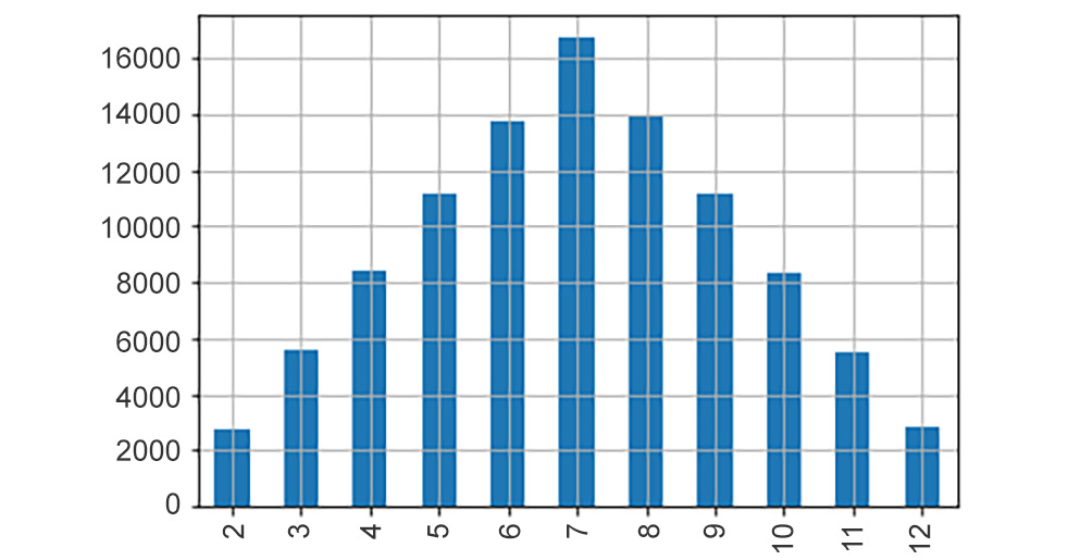
Figure 8.4: Frequencies of the values of X
We can see out of the 100,000 of X, it took the value 3 around 5,800 times and the value 6 a little less than 14,000 times, which is also very close to the number of times the value 8 appeared. We can also observe that the most common outcome was the number 7.
Following the relative frequency definition of probability, if we divide the frequencies by the number of values of X, we can get the probability of observing each of the values of X:
Prob_of_X_values = freq_of_X_values/X.shape[0]
Prob_of_X_values.sort_index().plot(kind='bar')
plt.grid();
This gives us the following plot:

Figure 8.5: Probability distribution of the values of X
The plot looks almost exactly like the last one, but in this case, we can see the probabilities of observing all the possible values of X. This is what we call the probability distribution (or simply the distribution) of a random variable: the probabilities of observing each of the values the random variable can take.
Let's illustrate both concepts, random variables and probability distribution, with another example. First, we'll define the random variable:
Y: Number of heads when tossing 10 fair coins.
Now, our task is to estimate the probability distribution. We know that this random variable can take 11 possible values: {0, 1, 2, 3, 4, 5, 6, 7, 8, 9, 10}. For each of these values, there is a corresponding probability that the Y variable will take that value. Intuitively, we know that it is very unlikely to observe extreme values of the variable: getting 10 heads (Y=10) or 10 tails (Y=0) is very unlikely. We also expect the Y variable to take values such as 4, 5, and 6 most of the time. We can calculate the probability distribution to validate our intuition.
Once again, let's simulate the experiment of tossing 10 coins. From there, we can observe the values of this random variable. Let's begin by simulating tossing 10 fair coins 1 million times:
np.random.seed(97)
ten_coins_a_million_times = np.random.randint(0, 2,
size=int(10e6))
.reshape(-1,10)
The preceding code will produce a matrix of 1,000,000 x 10, with each row representing the experiment of tossing 10 coins. We can consider 0s as tails and 1s as heads. Here, we have the first 12 rows:
ten_coins_a_million_times[:12, :]
The result is as follows:
array([[0, 1, 1, 1, 1, 1, 0, 1, 1, 0],
[0, 0, 1, 1, 1, 0, 1, 0, 0, 0],
[0, 1, 0, 1, 1, 0, 0, 0, 0, 1],
[1, 0, 1, 1, 0, 1, 0, 0, 1, 1],
[1, 0, 1, 0, 1, 0, 1, 0, 0, 0],
[0, 1, 1, 1, 0, 1, 1, 1, 1, 0],
[1, 1, 1, 1, 0, 1, 0, 1, 0, 1],
[0, 1, 0, 0, 1, 1, 1, 0, 0, 0],
[1, 0, 0, 1, 1, 1, 0, 0, 0, 0],
[0, 1, 0, 1, 0, 1, 0, 1, 0, 1],
[1, 0, 1, 1, 1, 0, 0, 0, 1, 0],
[0, 0, 0, 0, 1, 1, 1, 0, 1, 1]])
To produce the different values of Y, we need to add every row, like so:
Y = ten_coins_a_million_times.sum(axis=1)
Now, we can use the former calculated object (Y) to calculate probabilities of certain events, for instance, the probability of obtaining zero heads:
Prob_Y_is_0 = (Y == 0).sum() / Y.shape[0]
print(f'P(Y = 0) = {Prob_Y_is_0}')
The output is as follows:
P(Y = 0) = 0.000986
This is a very small number and is consistent with our intuition: it is very unlikely to get 10 tails. In fact, that only happened 986 times in 1 million experiments.
Just as we did previously, we can plot the probability distribution of Y:
Y = pd.Series(Y)
# counts the occurrences of each value
freq_of_Y_values = Y.value_counts()
Prob_of_Y_values = freq_of_Y_values/Y.shape[0]
Prob_of_Y_values.sort_index().plot(kind='bar')
plt.grid();
This is the output:

Figure 8.6: Probability distribution of Y
The probability of getting 5 heads is around 0.25, so around 25% of the time, we could expect to get 5 heads. The chance of getting 4 or 6 heads is also relatively high. What is the probability of getting 4, 5, or 6 heads? We can easily calculate this using Prob_of_Y_values by adding the respective probabilities of getting 4, 5, or 6 heads:
print(Prob_of_Y_values.loc[[4,5,6]])
print(f'P(4<=Y<=6) = {Prob_of_Y_values.loc[[4,5,6]].sum()}')
The result is as follows:
4 0.205283
5 0.246114
6 0.205761
dtype: float64
P(4<=Y<=6) = 0.657158
So, around 2/3 (~66%) of the time, we will observe 4, 5, or 6 heads when tossing 10 fair coins. Going back to the definition of probability as a measure of uncertainty, we could say that we are 66% confident that, when tossing 10 fair coins, we will see between 4 and 6 heads.
Exercise 8.02: Calculating the Average Wins in Roulette
In this exercise, we will learn how to use np.random.choice to simulate a real-world random process. Then, we will take this simulation and calculate how much money we will gain/lose on average if we play a large number of times.
We will simulate going to a casino to play roulette. European roulette consists of a ball falling on any of the integer numbers from 0 to 36 randomly with an equal chance of falling on any number. Many modalities of betting are allowed, but we will play it in just one way (which is equivalent to the famous way of betting on red or black colors). The rules are as follows:
- Bet m units (of your favorite currency) on the numbers from 19 to 36.
- If the outcome of the roulette is any of the selected numbers, then you win m units.
- If the outcome of the roulette is any number between 0 and 18 (inclusive), then you lose m units.
To simplify this, let's say the bets are of 1 unit. Let's get started:
- Import the NumPy library:
import numpy as np
- Use the np.random.choice function to write a function named roulette that simulates any number of games from European roulette:
def roulette(number_of_games=1):
# generate the Roulette numbers
roulette_numbers = np.arange(0, 37)
outcome = np.random.choice(a = roulette_numbers,
size = number_of_games,
replace = True)
return outcome
- Write a function named payoff that encodes the preceding payoff logic. It receives two arguments: outcome, a number from the roulette wheel (an integer from 0 to 36); and units to bet with a default value of 1:
def payoff(outcome, units=1):
# 1. Bet m units on the numbers from 19 to 36
# 2. If the outcome of the roulette is any of the
# selected numbers, then you win m units
if outcome > 18:
pay = units
else:
# 3. If the outcome of the roulette is any number
# between 0 and 18 (inclusive) then you lose m units
pay = -units
return pay
- Use np.vectorize to vectorize the function so it can also accept a vector of roulette outcomes. This will allow you to pass a vector of outcomes and get the respective payoffs:
payoff = np.vectorize(payoff)
- Now, simulate playing roulette 20 times (betting one unit). Use the payoff function to get the vector of outcomes:
outcomes = roulette(20)
payoffs = payoff(outcomes)
print(outcomes)
print(payoffs)
The output is as follows:
[29 36 11 6 11 6 1 24 30 13 0 35 7 34 30 7 36 32 12 10]
[ 1 1 -1 -1 -1 -1 -1 1 1 -1 -1 1 -1 1 1 -1 1 1 -1 -1]
- Simulate 1 million roulette games and use the outcomes to get the respective payoffs. Save the payoffs in a vector named payoffs:
number_of_games = int(1e6)
outcomes = roulette(number_of_games)
payoffs = payoff(outcomes)
- Use the np.mean function to calculate the mean of the payoffs vector. The value you will get should be close to -0.027027:
np.mean(payoffs)
The negative means that, on average, you lose -0.027027 for every unit you bet. Remember that your loss is the casino's profit. That is their business.
In this exercise, we learned how to simulate a real-world process using the capabilities of NumPy for random number generation. We also simulated a large number of events to get a long-term average.
Note
To access the source code for this specific section, please refer to https://packt.live/2AoiyGp.
You can also run this example online at https://packt.live/3irX6Si.
With that, we learned how we can make sense of random events by assigning probabilities to quantify uncertainty. Then, we defined some of the most important concepts in probability theory. We also learned how to assign probabilities to events using the relative frequency definition. In addition, we introduced the important concept of random variables. Computationally, we learned how to simulate values and samples with NumPy and how to use simulations to answer questions about the probabilities of certain events.
Depending on the types of values random variables can take, we can have two types:
- Discrete random variables
- Continuous random variables
We will provide some examples of both in the following two sections.
Discrete Random Variables
In this section, we'll continue learning about and working with random variables. We will study a particular type of random variable: discrete random variables. These types of variables arise in every kind of applied domain, such as medicine, education, manufacturing, and so on, and therefore it is extremely useful to know how to work with them. We will learn about perhaps the most important, and certainly one of the most commonly occurring, discrete distributions: the binomial distribution.
Defining Discrete Random Variables
Discrete random variables are those that can take only a specific number of values (technically, a countable number of values). Often, the values they can take are specific integer values, although this is not necessary. For instance, if a random variable can take the set of values {1.25, 3.75, 9.15}, it would also be considered a discrete random variable. The two random variables we introduced in the previous section are examples of discrete random variables.
Consider an example in which you are the manager of a factory that produces auto parts. The machine producing the parts will produce, on average, defective parts 4% of the time. We can interpret this 4% as the probability of producing defective parts. These auto parts are packaged in boxes containing 12 units, so, in principle, every box can contain anywhere from 0 to 12 defective pieces. Suppose we don't know which piece is defective (until it is used), nor do we know when a defective piece will be produced. Hence, we have a random variable. First, let's formally define it:
Z: number of defective auto parts in a 12-box pack.
As the manager of the plant, one of your largest clients asks you the following questions:
- What percentage of boxes have 12 non-defective pieces (zero defective pieces)?
- What percentage of boxes have 3 or more defective pieces?
You can answer both questions if you know the probability distribution for your variable, so you ask yourself the following:
What does the probability distribution of Z look like?
To answer this question, we can again use simulations. To simulate a single box, we can use np.random.choice and provide the probabilities via the p parameter:
np.random.seed(977)
np.random.choice(['defective', 'good'],
size=12, p=(0.04, 0.96))
The result is as follows:
array(['good', 'good', 'good', 'good', 'good', 'good', 'good',
'defective', 'good', 'good', 'good', 'good'], dtype='<U9')
We can see that this particular box contains one defective piece. Notice that the probability vector that was used in the function must add up to one: since the probability of observing a defective piece is 4% (0.04), the probability of observing a good piece is 100% – 4% = 96% (0.96), which are the values that are passed to the p argument.
Now that we know how to simulate a single box, to estimate the distribution of our random variable, let's simulate a large number of boxes; 1 million is more than enough. To make our calculations easier and faster, let's use 1s and 0s to denote defective and good parts, respectively. To simulate 1 million boxes, it is enough to change the size parameter to a tuple that will be of size 12 x 1,000,000:
np.random.seed(10)
n_boxes = int(1e6)
parts_per_box = 12
one_million_boxes = np.random.choice
([1, 0],
size=(n_boxes, parts_per_box),
p=(0.04, 0.96))
The first five boxes can be found using the following formula:
one_million_boxes[:5,:]
The output will be as follows:
array([[0, 1, 0, 0, 0, 0, 0, 0, 0, 0, 0, 0],
[1, 0, 0, 0, 0, 0, 0, 0, 0, 0, 0, 0],
[0, 0, 0, 0, 0, 0, 0, 0, 0, 0, 0, 0],
[0, 0, 0, 0, 0, 0, 0, 0, 0, 0, 0, 0],
[0, 0, 0, 0, 0, 0, 0, 0, 0, 0, 0, 0]])
Each of the zeros in the output represents a non-defective piece, and one represents a defective piece. Now, we count how many defective pieces we have per box, and then we can count how many times we observed 0, 1, 2, ..., 12 defective pieces, and with that, we can plot the probability distribution of Z:
# count defective pieces per box
defective_pieces_per_box = one_million_boxes.sum(axis=1)
# count how many times we observed 0, 1,…, 12 defective pieces
defective_pieces_per_box = pd.Series(defective_pieces_per_box)
frequencies = defective_pieces_per_box.value_counts()
# probability distribution
probs_Z = frequencies/n_boxes
Finally, let's visualize this:
print(probs_Z.sort_index())
probs_Z.sort_index().plot(kind='bar')
plt.grid()
The output will be as follows:
0 0.612402
1 0.306383
2 0.070584
3 0.009630
4 0.000940
5 0.000056
6 0.000004
7 0.000001
Here's what the probability distribution will look like:
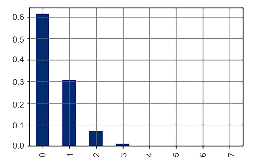
Figure 8.7: Probability distribution of Z
From this simulation, we can conclude that around 61% of boxes will be shipped with zero defective parts, and around 30% of the boxes will contain one defective part. We can also see that it is very, very unlikely to observe three or more defective parts in a box. Now, you can answer the questions your client had:
- What percentage of boxes have 12 non-defective parts? Answer: 61% of the boxes will contain 12 non-defective parts.
- What percentage of boxes have 3 or more defective pieces? Answer: Only about 1% of the boxes will contain 3 or more defective parts.
The Binomial Distribution
It turns out that, under certain conditions, we can find out the exact probability distribution of certain discrete random variables. The binomial distribution is a theoretical distribution that applies to random variables and fulfills the following three characteristics:
- Condition 1: For an individual observation, there are only two possible outcomes, usually denoted as success and failure. If the probability of success is p, then the probability of failure must be 1 – p.
- Condition 2: The experiment is performed a fixed number of times, usually denoted by n.
- Condition 3: All the experiments are independent, meaning that knowing the outcome of an experiment does not change the probability of the next. Therefore, the probability of success (and failure) remains the same.
If these conditions are met, then we say that the random variable follows a binomial distribution, or that the random variable is a binomial random variable. We can get the exact probability distribution of a binomial random variable, X, using the following formula:

Figure 8.8: Formula to calculate the probability distribution of X
Technically, the mathematical function that takes a possible value of a discrete random variable (x) and returns the respective probability is called the probability mass function. Notice that once we know the values of n and p from the previous equation, the probability depends only on the x value, so the former equation defines the probability mass function for a binomial random variable.
OK, this sounds and looks very theoretical and abstract (because it is). However, we have already introduced two random variables that follow the binomial distribution. Let's verify the conditions for the following:
Y: Number of heads when tossing 10 fair coins.
- Condition 1: For each individual coin, there are only two possible outcomes, head or tails, each with a fixed probability of 0.5. Since we were interested in the number of heads, heads can be considered our success and tails our failure.
- Condition 2: The number of coins was fixed at 10 coins.
- Condition 3: Each coin toss is independent: we implicitly (and logically) assumed that the outcome of one coin does not influence the outcome of any other coin.
So, we have the numbers we need to use in the preceding formula:
- p = 0.5
- n = 10
If we want to get the probability of getting five heads, then we only need to replace x = 5 in the formula with the known p and n:

Figure 8.9: Substituting the values of x, p and n in the probability distribution formula
Now, let's do these theoretical calculations with Python. It is time to introduce another Python module that we will be using heavily in this and the following chapter. The scipy.stats module contains many statistical functions. Among those, there are many that can be used to create random variables that follow many of the most commonly used probability distributions. Let's use this module to create a random variable that follows the theoretical binomial distribution. First, we instantiate the random variable with the appropriate parameters:
import scipy.stats as stats
Y_rv = stats.binom(
n = 10, # number of coins
p = 0.5 # probability of heads (success)
)
Once created, we can use the pmf method of this object to calculate the exact theoretical probabilities for each of the possible values Y can take. First, let's create a vector containing all the values Y can take (integers from 0 to 10):
y_values = np.arange(0, 11)
Now, we can simply use the pmf (which stands for probability mass function) method to get the respective probabilities for each of the former values:
Y_probs = Y_rv.pmf(y_values)
We can visualize the pmf we got like so:
fig, ax = plt.subplots()
ax.bar(y_values, Y_probs)
ax.set_xticks(y_values)
ax.grid()
The output we get is as follows:

Figure 8.10: pmf of Y
This looks very similar to what we got using the simulations. Now, let's compare both plots. We will create a DataFrame to make the plotting process easier:
Y_rv_df = pd.DataFrame({'Y_simulated_pmf': Prob_of_Y_values,
'Y_theoretical_pmf': Y_probs},
index=y_values)
Y_rv_df.plot(kind='bar')
plt.grid();
The output is as follows:

Figure 8.11: pmf of Y versus simulated results
The two sets of bars are practically identical; the probabilities we got from our simulation are very close to the theoretical values. This shows the power of simulations.
Exercise 8.03: Checking If a Random Variable Follows a Binomial Distribution
In this exercise, we will practice how to verify if a random variable follows a binomial distribution. We will also create a random variable using scipy.stats and plot the distribution. This will be a mostly conceptual exercise.
Here, we will check if the random variable, Z: number of defective auto parts in a 12-box pack, follows a binomial distribution (remember that we consider 4% of the auto parts are defective). Follow these steps to complete this exercise:
- Import NumPy, Matplotlib, and scipy.stats following the usual conventions:
import numpy as np
import scipy.stats as stats
import matplotlib.pyplot as plt
%matplotlib inline
- Just as we did in the Defining Discrete Random Variables section, try to conceptually check if Z fulfills the three characteristics given for a binomial random variable:
a. Condition 1: For each individual auto part, there are only two possible outcomes, defective or good. Since we were interested in the defective parts, then that outcome can be considered the success, with a fixed probability of 0.04 (4%).
b. Condition 2: The number of parts per box was fixed at 12, so the experiment was performed a fixed number of times per box.
c. Condition 3: We assumed that the defective parts had no relationship between one another because the machine randomly produces an average of 4% defective parts.
- Determine the p and n parameters for the distributions of this variable, that is, p = 0.04 and n = 12.
- Use the theoretical formula with the former parameters to get the exact theoretical probability of getting exactly one defective piece per box (using x = 1):

Figure 8.12: Substituting the values of x, p and n in the probability distribution formula
- Use the scipy.stats module to produce an instance of the Z random variable. Name it Z_rv:
# number of parts per box
parts_per_box = 12
Z_rv = stats.binom
(n = parts_per_box,
p = 0.04 # probability of defective piece (success)
)
- Plot the probability mass function of Z:
z_possible_values = np.arange(0, parts_per_box + 1)
Z_probs = Z_rv.pmf(z_possible_values)
fig, ax = plt.subplots()
ax.bar(z_possible_values, Z_probs)
ax.set_xticks(z_possible_values)
ax.grid();
The result looks like this:
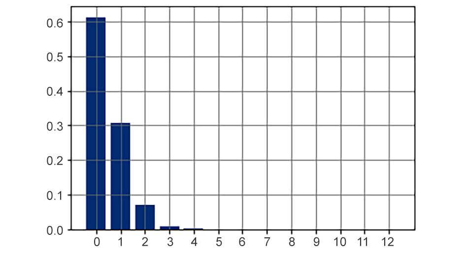
Figure 8.13: pmf of Z
In this exercise, we learned how to check for the three conditions that are needed for a discrete random variable to have a binomial distribution. We concluded that the variable we analyzed indeed has a binomial distribution. We were also able to calculate its parameters and use them to create a binomial random variable using scipy.stats and plotted the distribution.
Note
To access the source code for this specific section, please refer to https://packt.live/3gbTm5k.
You can also run this example online at https://packt.live/2Anhx1k.
In this section, we focused on discrete random variables. Now, we know they are the kind of random variables that can take on a specific number of values. Typically, these are integer values. Often, these types of variables are related to counts: the number of students that will pass a test, the number of cars crossing a bridge, and so on. We also learned about the most important distribution of discrete random variables, known as the binomial distribution, and how we can get the exact theoretical probabilities of a binomial random variable using Python.
In the next section, we'll focus on continuous random variables.
Continuous Random Variables
In this section, we'll continue working with random variables. Here, we'll discuss continuous random variables. We will learn the key distinction between continuous and discrete probability distributions. In addition, we will introduce the mother of all distributions: the famous normal distribution. We will learn how to work with this distribution using scipy.stats and review its most important characteristics.
Defining Continuous Random Variables
There are certain random quantities that, in principle, can take any real value in an interval. Some examples are as follows:
- The price of the IBM stocks one week from now
- The number of calories ingested by a person in a day
- The closing exchange rate between the British pound and the Euro
- The height of a randomly chosen male from a specific group
Because of their nature, these variables are known as continuous random variables. As with discrete random variables, there are many theoretical distributions that can be used to model real-world phenomena.
To introduce this type of random variable, let's look at an example we are already familiar with. Once again, let's load the games dataset we introduced in Chapter 7, Doing Basic Statistics with Python:
games = pd.read_csv('./data/appstore_games.csv')
original_colums_dict = {x: x.lower().replace(' ','_')
for x in games.columns}
# renaming columns
games.rename(columns = original_colums_dict, inplace = True)
One of the variables we have in the dataset is size of the game in bytes. Before visualizing the distribution of this variable, we will transform it into megabytes:
games['size'] = games['size']/(1e6)
# replacing the one missing value with the median
games['size'] = games['size'].fillna(games['size'].median())
games['size'].hist(bins = 50, ec='k');
The output is as follows:
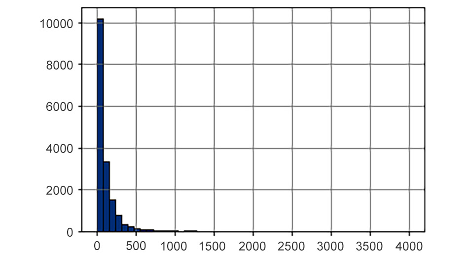
Figure 8.14: Distribution of the size of the game
Let's define our random variable, X, as follows:
X: Size of a randomly chosen strategy game from the app store.
Having defined this random variable, we can start asking questions about the probabilities of certain events:
- P(X > 100): Probability that X is strictly greater than 100 MB
- P(100 ≤ X ≤ 400): Probability that X is between 100 and 400 MB
- P(X = 152.53): Probability of X being exactly 152.53 MB
By now, you know how you can estimate these probabilities by using the relative frequency definition of probability: count the number of times an event happens and divide this by the total number of events (games, in this case):
# get the number of games to use as denominator
number_of_games = games['size'].size
# calculate probabilities
prob_X_gt_100 = (games['size'] > 100).sum()/number_of_games
prob_X_bt_100_and_400 = ((games['size'] >= 100) &
(games['size'] <= 400))
.sum()/number_of_games
prob_X_eq_152_53 = (games['size'] == 152.53).sum()/number_of_games
# print the results
print(f'P(X > 100) = {prob_X_gt_100:0.5f}')
print(f'P(100 <= X <= 400) = {prob_X_bt_100_and_400:0.5f}')
print(f'P(X = 152.53) = {prob_X_eq_152_53:0.5f}')
The results are as follows:
P(X > 100) = 0.33098
P(100 <= X <= 400) = 0.28306
P(X = 152.53) = 0.00000
Notice the last probability we calculated, P(X = 152.53). The estimated probability that a random variable takes a specific value (such as 152.53) is zero. This is always the case for any continuous random variable. Since these types of variables can, in principle, take an infinite number of values, then the probability of taking exactly a specific value must be zero.
The preceding example shows that when we have enough data points about a continuous random variable, we can use the data to estimate the probability of the random variable taking values within certain intervals. However, having lots of observations about one variable might not always be the case. Given this fact, let's consider the following questions:
- What if we have no data at all?
- What if we don't have enough data?
- Can we perform simulations to get an estimation of the probabilities of certain events (as we did with discrete random variables)?
These are sensible questions, and we can answer them by knowing more about theoretical continuous probability distributions:
- What if we have no data at all? We can make some reasonable assumptions about the variable, and then model it using one of the many theoretical continuous probability distributions.
- What if we don't have enough data? We can make some reasonable assumptions about the variable, support these assumptions with the data, and use estimation techniques (the subject of the next chapter) to estimate the parameters of the chosen theoretical continuous probability distribution.
- Can we perform simulations to get an estimation of the probabilities of certain events (as we did with discrete random variables)? Yes. Once we have chosen the probability distribution, along with its parameters, we can use simulations to answer complicated questions.
To make the previous answers clear, in the following subsections, we'll introduce the most important continuous probability distribution: the normal distribution.
It is worth noting that for continuous random variables, the probability distribution is also known as the probability density function or pdf.
The Normal Distribution
Let's introduce the most famous and important distribution in probability theory: the normal distribution. The pdf of the normal distribution is defined by the following equation:

Figure 8.15: The pdf of the normal distribution
Here, π and e are the well-known mathematical constants. Don't try to understand the equation; all you need to know is two things: first, that the distribution is completely determined when we have two parameters:
- µ: The mean of the distribution
- σ: The standard deviation of the distribution
Second, if X is a random variable that follows a normal distribution, then for a possible value x, the preceding formula will give you a value that is directly related to the probability of the variable taking values near x. Unlike the formula of the binomial distribution, where we got the probability by directly plugging the value, x, into the formula, in the case of continuous random variables, it is different: there is no direct interpretation of the values given by the formula. The following example will clarify this.
We will create a random variable that follows a normal distribution using the scipy.stats module. Let's suppose that the heights of a certain population of males is described by a normal distribution with a mean of 170 cm and a standard deviation of 10 cm. To create this random variable using scipy.stats, we need to use the following code:
# set the mu and sigma parameters of the distribution
heights_mean = 170
heights_sd = 10
# instantiate the random variable object
heights_rv = stats.norm(
loc = heights_mean, # mean of the distribution
scale = heights_sd # standard deviation
)
The preceding code creates the normally distributed random variable, whose pdf looks like this:

Figure 8.16: The pdf of a normally distributed random variable
For every value, x, say, 175, we can get the value of the pdf by using the pdf method, like so:
heights_rv.pdf(175)
The result is as follows:
0.03520653267642
This number is what you would get if you replaced x with 175 in the preceding formula:
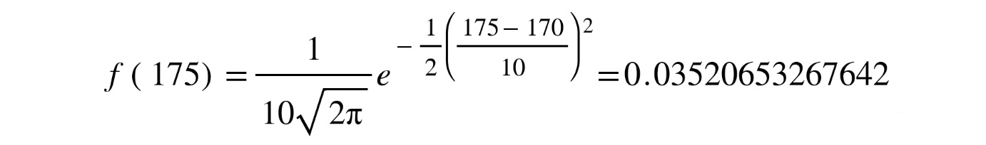
Figure 8.17 Substituting the vale of x=175
To be clear, this is not the probability of observing a male whose height is 175 cm (remember that the probability of this variable taking a specific value should be zero) as this number does not have a simple direct interpretation. However, if we plot the whole density curve, then we can start understanding the distribution of our random variable. To plot the whole probability density function, we must create a vector that contains a collection of possible values that this variable can take. According to the context of male heights, let's say that we want to plot the pdf for values between 130 cm and 210 cm, which are the likely values for healthy male adults. First, we create the vector of values using np.linspace, which in this case will create 200 equally spaced numbers between 120 and 210 (inclusive):
values = np.linspace(130, 210, num=200)
Now, we can produce the pdf and plot against the created values:
heights_rv_pdf = heights_rv.pdf(values)
plt.plot(values, heights_rv_pdf)
plt.grid();
The curve looks like this:
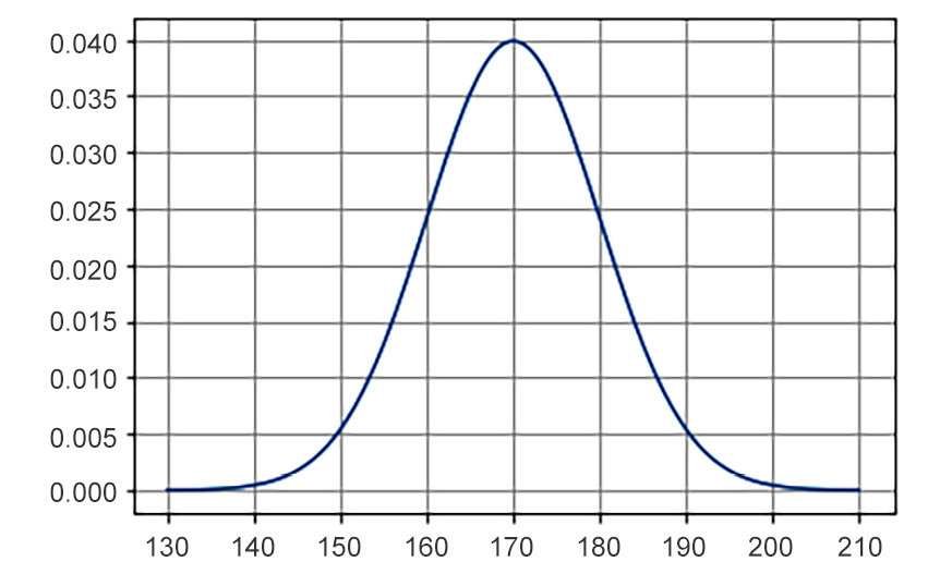
Figure 8.18: Example of a normal distribution with mean=170 and sd=10
The higher the curve, the more likely it is to observe those values around the corresponding x axis value. For instance, we can see that we are more likely to observe male heights between 160 cm and 170 cm than those between 140 cm and 150 cm.
Now that we have defined this normally distributed random variable, can we use simulations to answer certain questions about it? Absolutely. In fact, now, we will learn how to use the already defined random variable to simulate sample values. We can use the rvs method for this, which generates random samples from the probability distribution:
sample_heighs = heights_rv.rvs
(size = 5,
random_state = 998 # similar to np.seed)
for i, h in enumerate(sample_heighs):
print(f'Men {i + 1} height: {h:0.1f}')
The result is as follows:
Men 1 height: 171.2
Men 2 height: 173.3
Men 3 height: 157.1
Men 4 height: 164.9
Men 5 height: 179.1
Here, we are simulating taking five random males from the population and measuring their heights. Notice that we used the random_state parameter, which plays a similar role to the numpy.seed: it ensures anyone running the same code will get the same random values.
As we did previously, we can use the simulations to answer questions about the probability of events related to this random variable. For instance, what is the probability of finding a male taller than 190 cm? The following code calculates this simulation using our previously defined random variable:
# size of the simulation
sim_size = int(1e5)
# simulate the random samples
sample_heights = heights_rv.rvs
(size = sim_size,
random_state = 88 # similar to np.seed)
Prob_event = (sample_heights > 190).sum()/sim_size
print(f'Probability of a male > 190 cm: {Prob_event:0.5f}
(or {100*Prob_event:0.2f}%)')
The result is:
Probability of a male > 190 cm: 0.02303 (or 2.30%)
As we will see in the following section, there is a way to get the exact probabilities from the density function without the need to simulate values, which can sometimes be computationally expensive and unnecessary.
Some Properties of the Normal Distribution
One impressive fact about the universe and mathematics is that many variables in the real world follow a normal distribution:
- Human heights
- Weights of members of most species of mammals
- Scores of standardized tests
- Deviations from product specifications in manufacturing processes
- Medical measurements such as diastolic pressure, cholesterol, and sleep times
- Financial variables such as the returns of some securities
The normal distribution describes so many phenomena and is so extensively used in probability and statistics that it is worth knowing two key properties:
- The normal distribution is completely determined by its two parameters: mean and standard deviation.
- The empirical rule of a normally distributed random variable tells us what proportion of observations that we will find, depending on the number of standard deviations away from the mean.
Let's understand these two key properties. First, we will illustrate how the parameters of the distribution determine its shape:
- The mean determines the center of the distribution.
- The standard deviation determines how wide (or spread out) the distribution is.
To illustrate this property, let's say that we have the following three populations of male heights. Each population correspond to a different country:
- Country A: Mean = 170 cm, standard deviation = 10 cm
- Country B: Mean = 170 cm, standard deviation = 5 cm
- Country C: Mean = 175 cm, standard deviation = 10 cm
With these parameters, we can visualize and contrast the distributions of the three different countries. Before visualizing, let's create the random variables:
# parameters of distributions
heights_means = [170, 170, 175]
heights_sds = [10, 5, 10]
countries = ['Country A', 'Country B', 'Country C']
heights_rvs = {}
plotting_values = {}
# creating the random variables
for i, country in enumerate(countries):
heights_rvs[country] = stats.norm(
loc = heights_means[i], # mean of the distribution
scale = heights_sds[i] # standard deviation
)
With these objects created, we can proceed with the visualizations:
# getting x and y values for plotting the distributions
for i, country in enumerate(countries):
x_values = np.linspace(heights_means[i] - 4*heights_sds[i],
heights_means[i] + 4*heights_sds[i])
y_values = heights_rvs[country].pdf(x_values)
plotting_values[country] = (x_values, y_values)
# plotting the three distributions
fig, ax = plt.subplots(figsize = (8, 4))
for i, country in enumerate(countries):
ax.plot(plotting_values[country][0],
plotting_values[country][1],
label=country, lw = 2)
ax.set_xticks(np.arange(130, 220, 5))
plt.legend()
plt.grid();
The plot looks like this:
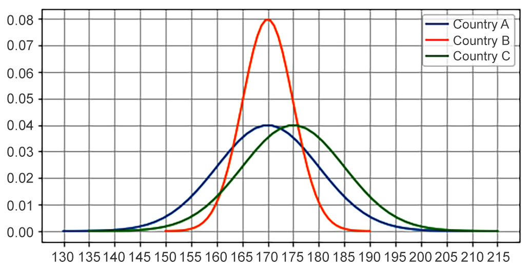
Figure 8.19: Comparison of normal distributions with different parameters
Although the populations for Country A and Country B have the same mean (170 cm), the difference in standard deviations implies that the distribution for Country B is much more concentrated around 170 cm. We could say that the males in this country tend to have more homogenous heights. The curves for Country A and Country C are basically the same; the only difference is that the curve for Country C is shifted to the right by 5 cm, which implies that it would be more likely to find males around 190 cm in height and above in Country C than in Country A or Country B (the green curve has a greater y axis value than the other two at x=190 and above).
The second important characteristic of the normal distribution is known as the empirical rule. Let's take our example of the population of male heights that are normally distributed with a mean of 170 cm and a standard deviation of 10 cm:
- ~68% of observations will lie in the interval: mean ± 1 sd. For the height of males, we will find that around 68% of males are between 160 cm and 180 cm (170 ± 10) in height.
- ~95% of observations will lie in the interval: mean ± 2 sd. For the height of males, we will find that around 95% of males are between 150 cm and 190 cm (170 ± 20) in height.
- More than 99% of observations will lie in the interval: mean ± 3 sd. Virtually all observations will be at a distance that is less than three standard deviations from the mean. For the height of males, we will find that around 99.7% of males will be between 150 cm and 200 cm (170 ± 30) in height.
The empirical rule can be used to quickly give us a sense of the proportion of observations we expect to see when we consider some number of standard deviations from the mean.
To finish this section and this chapter, one very important fact you should know about any continuous random variable is that the area under the probability distribution will give the probability of the variable being in a certain range. Let's illustrate this with the normal distribution, and also connect this with the empirical rule. Say we have a normally distributed random variable with mean = 170 and standard deviation = 10. What is the area under the probability distribution between x = 160 and x = 180 (one standard deviation away from the mean)? The empirical rule tells us that 68% of the observations will lie in this interval, so we would expect that ![]() , which will correspond with the area below the curve in the interval [160, 180]. We can visualize this plot with matplotlib. The code to produce the plot is somewhat long, so we will split it into two parts. First, we will create the function to plot, establish the limits of the plots in the x axis, and define the vectors to plot:
, which will correspond with the area below the curve in the interval [160, 180]. We can visualize this plot with matplotlib. The code to produce the plot is somewhat long, so we will split it into two parts. First, we will create the function to plot, establish the limits of the plots in the x axis, and define the vectors to plot:
from matplotlib.patches import Polygon
def func(x):
return heights_rv.pdf(x)
lower_lim = 160
upper_lim = 180
x = np.linspace(130, 210)
y = func(x)
Now, we will create the figure with a shaded region:
fig, ax = plt.subplots(figsize=(8,4))
ax.plot(x, y, 'blue', linewidth=2)
ax.set_ylim(bottom=0)
# Make the shaded region
ix = np.linspace(lower_lim, upper_lim)
iy = func(ix)
verts = [(lower_lim, 0), *zip(ix, iy), (upper_lim, 0)]
poly = Polygon(verts, facecolor='0.9', edgecolor='0.5')
ax.add_patch(poly)
ax.text(0.5 * (lower_lim + upper_lim), 0.01,
r"$int_{160}^{180} f(x)mathrm{d}x$",
horizontalalignment='center', fontsize=15)
fig.text(0.85, 0.05, '$height$')
fig.text(0.08, 0.85, '$f(x)$')
ax.spines['right'].set_visible(False)
ax.spines['top'].set_visible(False)
ax.xaxis.set_ticks_position('bottom')
ax.set_xticks((lower_lim, upper_lim))
ax.set_xticklabels(('$160$', '$180$'))
ax.set_yticks([]);
The output will be as follows:

Figure 8.20: Area under the pdf as the probability of an event
How do we calculate the integral that will give us the area under the curve? The scipy.stats module will make this very easy. Using the cdf (cumulative distribution function) method of the random variable, which is essentially the integral of the pdf, we can easily evaluate the integral by subtracting the lower and upper limits (remember the fundamental theorem of calculus):
# limits of the integral
lower_lim = 160
upper_lim = 180
# calculating the area under the curve
Prob_X_in_160_180 = heights_rv.cdf(upper_lim) -
heights_rv.cdf(lower_lim)
# print the result
print(f'Prob(160 <= X <= 180) = {Prob_X_in_160_180:0.4f}')
The result is as follows:
Prob(160 <= X <= 180) = 0.6827
And this is how we get probabilities from the pdf without the need to perform simulations. Let's look at one last example to make this clear by connecting it with an earlier result. A few pages earlier, for the same population, we asked, What is the probability of finding a male taller than 190 cm? We got the answer by performing simulations. Now, we can get the exact probability like so:
# limits of the integral
lower_lim = 190
upper_lim = np.Inf # since we are asking X > 190
# calculating the area under the curve
Prob_X_gt_190 = heights_rv.cdf(upper_lim) -
heights_rv.cdf(lower_lim)
# print the result
print(f'Probability of a male > 190 cm: {Prob_X_gt_190:0.5f}
(or {100*Prob_X_gt_190:0.2f}%)')
The result is as follows:
Probability of a male > 190 cm: 0.02275 (or 2.28%)
If you compare this with the result we got earlier, you will see it is virtually the same. However, this approach is better since it's exact and does not require us to perform any computationally heavy or memory-consuming simulations.
Exercise 8.04: Using the Normal Distribution in Education
In this exercise, we'll use a normal distribution object from scipy.stats and the cdf and its inverse, ppf, to answer questions about education.
In psychometrics and education, it is a well-known fact that many variables relevant to education policy are normally distributed. For instance, scores in standardized mathematics tests follow a normal distribution. In this exercise, we'll explore this phenomenon: in a certain country, high school students take a standardized mathematics test whose scores follow a normal distribution with the following parameters: mean = 100, standard deviation = 15. Follow these steps to complete this exercise:
- Import NumPy, Matplotlib, and scipy.stats following the usual conventions:
import numpy as np
import scipy.stats as stats
import matplotlib.pyplot as plt
%matplotlib inline
- Use the scipy.stats module to produce an instance of a normally distributed random variable, named X_rv, with mean = 100 and standard deviation = 15:
# producing the normal distribution
X_mean = 100
X_sd = 15
# create the random variable
X_rv = stats.norm(loc = X_mean, scale = X_sd)
- Plot the probability distribution of X:
x_values = np.linspace(X_mean - 4 * X_sd, X_mean + 4 * X_sd)
y_values = X_rv.pdf(x_values)
plt.plot(x_values, y_values, lw=2)
plt.grid();
The output will be as follows:
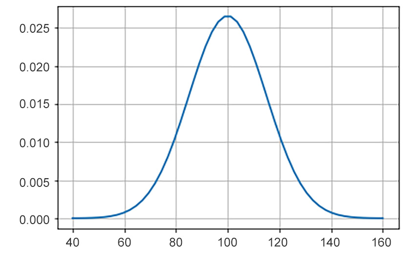
Figure 8.21: Probability distribution of tests scores
- The Ministry of Education has decided that the minimum score for someone to be considered competent in mathematics is 80. Use the cdf method to calculate the proportion of students that will get a score above that score:
Prob_X_gt_80 = X_rv.cdf(np.Inf) - X_rv.cdf(80)
print(f'Prob(X >= 80): {Prob_X_gt_80:0.5f}
(or {100*Prob_X_gt_80:0.2f}%)')
The result is as follows:
Prob(X >= 80): 0.90879 (or 90.88%)
Around 91% of the students are considered competent in mathematics.
- A very selective university wants to set very high standards for high school students that are admitted to their programs. The policy of the university is to only admit students with mathematics scores in the top 2% of the population. Use the ppf method (which is essentially the inverse function of the cdf method) with an argument of 1 - 0.02 = 0.98 to get the cut-off score for admission:
proportion_of_admitted = 0.02
cut_off = X_rv.ppf(1-proportion_of_admitted)
print(f'To admit the top {100*proportion_of_admitted:0.0f}%,
the cut-off score should be {cut_off:0.1f}')
top_percents = np.arange(0.9, 1, 0.01)
The result should be as follows:
To admit the top 2%, the cut-off score should be 130.8
In this exercise, we used a normal distribution and the cdf and ppf methods to answer real-world questions about education policy.
Note
To access the source code for this specific section, please refer to https://packt.live/3eUizB4.
You can also run this example online at https://packt.live/2VFyF9X.
In this section, we learned about continuous random variables, as well as the most important distribution of these types of variables: the normal distribution. The key takeaway from this section is that a continuous random variable is determined by its probability density function, which is, in turn, determined by its parameters. In the case of the normal distribution, its two parameters are the mean and the standard deviation. We used an example to demonstrate how these parameters influence the shape of the distribution.
Another important takeaway is that you can use the area below the pdf to calculate the probability of certain events. This is true for any continuous random variable, including, of course, those that follow a normal distribution.
Finally, we also learned about the empirical rule for the normal distribution, which is a good-to-know rule of thumb if you want to quickly get a sense of the proportion of values that will lie k standard deviations away from the mean of the distribution.
Now that you are familiar with this important distribution, we will continue using it in the next chapter when we encounter it again in the context of the central limit theorem.
Activity 8.01: Using the Normal Distribution in Finance
In this activity, we'll explore the possibility of using the normal distribution to understand the daily returns of the stock price. By the end of this activity, you should have an opinion regarding whether the normal distribution is an appropriate model for the daily returns of stocks.
In this example, we will use daily information about Microsoft stock provided by Yahoo! Finance. Follow these steps to complete this activity:
Note
The dataset that's required to complete this activity can be found at https://packt.live/3imSZqr.
- Using pandas, read the CSV file named MSFT.csv from the data folder.
- Optionally, rename the columns so they are easy to work with.
- Transform the date column into a proper datetime column.
- Set the date column as the index of the DataFrame.
- In finance, the daily returns of a stock are defined as the percentage change of the daily closing price. Create the returns column in the MSFT DataFrame by calculating the percent change of the adj close column. Use the pct_change series pandas method to do so.
- Restrict the analysis period to the dates between 2014-01-01 and 2018-12-31 (inclusive).
- Use a histogram to visualize the distribution of the returns column, using 40 bins. Does it look like a normal distribution?
The output should look like this:
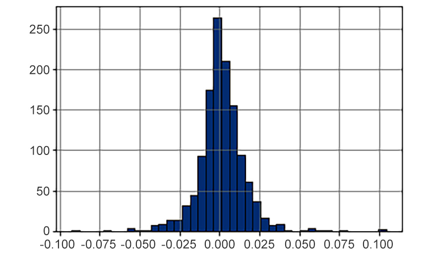
Figure 8.22: Histogram of returns of the MSFT stock
- Calculate the descriptive statistics of the returns column:
count 1258.000000
mean 0.000996
std 0.014591
min -0.092534
25% -0.005956
50% 0.000651
75% 0.007830
max 0.104522
Name: returns, dtype: float64
- Create a random variable named R_rv that will represent The daily returns of the MSFT stock. Use the mean and standard deviation of the return column as the parameters for this distribution.
- Plot the distribution of R_rv and the histogram of the actual data. Then, use the plt.hist() function with the density=True parameter so that both the real data and the theoretical distribution appear in the same scale:

Figure 8.23: Histogram of returns of the MSFT stock
- After looking at the preceding plot, would you say that the normal distribution provides an accurate model for the daily returns of Microsoft stock?
- Additional activity: Repeat the preceding steps with the PG.csv file, which contains information about the Procter and Gamble stock.
This activity was about observing real-world data and trying to use a theoretical distribution to describe it. This is important because by having a theoretical model, we can use its known properties to arrive at real-world conclusions and implications. For instance, you could use the empirical rule to say something about the daily returns of a company, or you could calculate the probability of losing a determined amount of money in a day.
Note
The solution for this activity can be found on page 684.
Summary
This chapter gave you a brief introduction to the branch of mathematics regarding probability theory.
We defined the concept of probability, as well as some of its most important rules and associated concepts such as experiment, sample space, and events. We also defined the very important concept of random variables and provided examples of the two main discrete and continuous random variables. Later in this chapter, we learned how to create random variables using the scipy.stats module, which we also used to generate the probability mass function and the probability density function. We also talked about two of the most important random variables in the (literal) universe: the normal distribution and the binomial distribution. These are used in many applied fields to solve real-world problems.
This was, of course, a brief introduction to the topic, and the goal was to present and make you familiar with some of the basic and foundational concepts in probability theory, especially those that are crucial and necessary to understand and use inferential statistics, which is the topic of the next chapter.
WUE84
JNP97