CHAPTER 5

The CDS Basis II: Further Analysis of the Cash and Synthetic Credit Market Differential

In the previous chapter, we described the traditional method of calculating the credit default swap (CDS) basis. For accurate analysis, this is now regarded as misleading, especially when bond prices are trading above or below par. Investors often require more effective measures of the basis. In this chapter, we assess why the common measure of the basis is inappropriate in certain cases, before considering alternative measures that should better suit investors' purposes. We conclude that an adjusted Z-spread, based on default probabilities implied by credit default swap prices, is the best measure to use when calculating the basis.

Basis and Relative Value

A basis exists in every market where cash and derivatives on the cash are traded. The cash-CDS basis is the difference in value between the CDS market and the cash bond market. The existence of a non–zero basis implies potential trading gains of either of the following:

Negative basis: where there is a relatively low spread in the CDS market and a higher spread for the cash bond. That is, in relative terms, the bond is cheap and the CDS is dear. In a negative basis strategy, which is effected by buying the cash bond and buying protection on the same name, the trader aims to earn a risk-free return by buying and selling identical credit risk but across two different markets.

Positive basis: effected by selling the cash bond and selling CDS protection on the same name, with the aim of exploiting a relatively low value CDS price and a low spread (high price) bond value.

For reasons of transparency and accessibility, investors require a measurement of value that is relative to Libor. With a CDS contract, there is only one measure of value, the “spread,” and so no uncertainty as to which measure is the correct one. With cash bonds, however, the quoted price can be translated into more than one Libor spread—namely, the interpolated spread, asset-swap spread (ASW), yield-to-maturity spread over swaps, and the Z-spread. The choice of which Libor spread to use therefore becomes central to the issue of basis measurement.

Basis Spread Measures

A wide range of factors drives the basis. These factors were described in detail in Chapter 3. The existence of a non–zero basis has implications for investment strategy. For instance, when the basis is negative, investors may prefer to hold the cash bond; whereas if—for liquidity, supply, or other reasons—the basis is positive, the investor may wish to hold the asset synthetically, by selling protection using a credit default swap. Another approach is to arbitrage between the cash and synthetic markets, in the case of a negative basis by buying the cash bond and shorting it synthetically by buying protection in the CDS market. Investors have a range of spreads to use when performing their relative value analysis.

Because the synthetic market in credit is often viewed to be a reliable indicator of the cash market in credit, it is important for all market participants to be familiar with the two-way relationship between the two markets. The relationship is represented by the credit default swap basis: a measure of the difference in price and value between the cash and synthetic credit markets. An accurate measure of the basis is vital for an effective assessment of the relationship between the two markets to be made.

ASW Spread

The potential to create an opportunity for arbitrage trading between the cash and synthetic markets means that often the basis is actually quite small in size. This infrequency of opportunity, however, means that it is vital to obtain an accurate measure. The traditional method used to calculate the basis given by equation (3.1) in Chapter 3 can be regarded as being of sufficient accuracy only if the following conditions are satisfied:

• The CDS and bond are of matching maturities;
• For many reference names, both instruments carry a similar level of subordination.

The conventional approach for analyzing an asset swap uses the bond's yield-to-maturity (YTM) in calculating the spread. The assumptions implicit in the YTM calculation make this spread problematic for relative analysis.

The most critical issue, however, is the nature of the construction of the asset-swap structure itself: the need for the cash bond price to be priced at or very near to par. Most corporate bonds trade significantly away from par, thus rendering the par asset-swap price an inaccurate measure of their credit risk. The standard asset swap is constructed as a par product; hence, if the bond being asset-swapped is trading above par, then the swap price will overestimate the level of credit risk. If the bond is trading below par, the asset swap will underestimate the credit risk associated with the bond. We see, then, that using the CDS-ASW method will provide an unreliable measure of the basis. We therefore need to use another methodology for measuring the basis.

Z-Spread

A commonly used alternative to the ASW spread is the Z-spread. The Z-spread uses the zero-coupon yield curve to calculate spread, so in theory is a more effective spread to use. The zero-coupon curve used in the calculation is derived from the interest-rate swap curve. Put simply, the Z-spread is the basis-point spread that would need to be added to the implied spot yield curve such that the discounted cash flows of a bond are equal to its present value (its current market price). Each bond cash flow is discounted by the relevant spot rate for its maturity term. How does this differ from the conventional asset-swap spread? Essentially, in its use of zero-coupon rates when assigning a value to a bond. Each cash flow is discounted using its own particular zero-coupon rate. A bond's price at any time can be taken to be the market's value of the bond's cash flows. Using the Z-spread, we can quantify what the swap market thinks of this value—that is, by how much the conventional spread differs from the Z-spread. Both spreads can be viewed as the coupon of a swap market annuity of equivalent credit risk of the bond being valued.

The Z-spread was described in detail in Chapter 2.

In practice, the Z-spread, especially for shorter-dated bonds and for higher-credit-quality bonds, does not differ greatly from the conventional asset-swap spread. The Z-spread is usually the higher spread of the two, following the logic of spot rates, but not always. If it differs greatly, then the bond can be considered to be mispriced.

Critique of the Z-Spread

Although the Z-spread is an improved value to use when calculating the basis compared to the ASW spread, it is not a direct comparison with a CDS premium. This is because it does not allow for probability of default—or, more specifically, timing of default. The Z-spread uses the correct zero-coupon rates to discount each bond cash flow, but it does not reflect the fact that, as coupons are received over time, each cash flow will carry a different level of credit risk. In fact, each cash flow will represent different levels of credit risk.

Given that a corporate bond that pays a spread over Treasuries or Libor must, by definition, be assumed to carry credit risk, we need to incorporate a probability of default factor if we compare its value to that of the same-name CDS. If the bond defaults, investors expect to receive a proportion of their holding back; this amount is given by the recovery rate. If the probability of default is p, then investors will receive the recovery rate amount after default. Prior to this, they will receive (1 − p). To gain an accurate measure of the basis therefore, we should incorporate this probability of default factor.

Adjusted Z-Spread

For the most accurate measure of the basis when undertaking relative value strategy, investors should employ the adjusted Z-spread, sometimes known as the C-spread. With this methodology, cash flows are adjusted by their probability of being paid. Because the default probability will alter over time, a static value cannot be used, so the calculation is done using a binomial approach, with the relevant default probability for each cash-flow pay date. An adjusted Z-spread can be calculated by either converting the bond price to a CDS-equivalent price, or converting a CDS spread to a bond-equivalent price. This is then subtracted from the CDS spread to give the adjusted basis.

Analyzing the Basis

We wish to formulate a framework by which we can “price” the basis, in effect a more effective method to analyze the basis beyond the first-generation principles outlined in Choudhry (2004). This requires that we understand the behavior and characteristics of the CDS as a hedging instrument.

Simplified Approach

All else being equal, under equation (3.1), we would expect the basis to be negative, due to the financing costs associated with the cash bond position. In practice, as we saw in Chapter 3, a wide range of technical and market factors drives the basis, and it is more common to observe a positive basis. When considering the basis, the coupon level on the cash bond is key to the analysis and also drives the basis. Bonds will trade above par when their coupon is high relative to current interest rates (given by swap rates); they trade below par when the opposite occurs. When above par, asset-swap spreads should be expected to lie above CDS premiums and so drive the basis downward, and vice versa when the bond price is below par. In addition, the CDS exhibits convexity, since the profit and loss on a CDS position does not move in direct proportion to the change in the credit spread. This is illustrated in FIGURE 5.1. Because this is not the case for asset-swap values, especially at higher credit spreads, we take this into account when pricing the basis.

FIGURE 5.1 CDS convexity

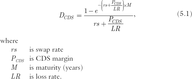
To value the basis, then, we want to account for the instruments' convexity. We use the instruments' duration in this analysis, a value required if calculating the position p&l. An effective approximation of CDS duration is given by

We noted there are two approaches to equate CDS premiums with bond prices. One approach is to value the bond using CDS reference prices. To do this, we need to transform the latter into a synthetic bond, and then use this synthetic bond value to calculate the basis. This produces more of a “like-for-like” spread that we can then compare to the cash spread.

We require therefore the asset-swap spread, obtained from the CDS duration as follows:

In other words, we can calculate the asset-swap spread directly from the CDS of similar maturity. The simplified model shown above is straightforward to calculate, and focuses on the two main factors that make basis calculation problematic: the convexity effects of CDSs compared to bonds, and the coupon effects of bonds being priced away from par. With the former, as CDS spreads widen, their duration decreases, so that bond spreads narrow relative to CDS spreads. With the latter, the higher the coupon relative to market rates (given by the swap rate for the same maturity), the wider will be the asset-swap spread relative to CDSs.

Unfortunately, the simple model is not practical because coupons are not continuously compounded and so require adjustment. Also, there is not always a bond and CDS of near-similar maturities to use in comparison. We therefore adopt another approach.

Pricing the Basis

Given the shortcomings of the methods described up to now, we wish to apply a technique that enables us to calculate the basis more effectively, on a more “like-for-like” level. Remember, we have two sources of credit-risk pricing: the cash bond yield and the CDS premium. When making the comparison between the two markets, we need to adjust one before comparing to the other, hence the name “adjusted basis” or “adjusted Z-spread.” To calculate the basis, then, we can do one of the following:

• Calculate the cash bond spread given by the CDS term structure; that is, price the bond according to the CDS curve and compare this spread to the bond market spread; or
• Calculate the CDS price given by the bond yield curve; that is, price the CDS on the bond curve and then compare it to the CDS market price.

In theory, the basis should be the same whichever approach is used.

Either approach can be adopted in principle, although the first approach is more problematic because the bond price (yield) does not make explicit which term default probability it is that is being priced. Under the latter approach, we can use the CDS term structure to build a default probability curve. We look at both approaches in the next section; first, we examine the theoretical background.

General Pricing Framework

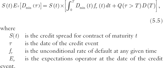
We need to set first the relationships for CDS and bond pricing. With a CDS, the contract is terminated on occurrence of a credit event, with settlement taking place upon payment of the accrued premium.

If

is the duration of an interest-rate swap of maturity t, and T is the fixed-rate payment dates, then we therefore write the duration of the CDS contract at the termination date as

The net present value (NPV) of the CDS fixed-rate premiums is given by

We assume that a credit event is a default and vice versa. In fact, the NPV is given by multiplying the CDS spread by the CDS duration D_CDS.

The NPV of the protection payment on occurrence of credit event, which we denote as the CDS floating-rate payment, is given by

where

RR is the recovery rate, usually assumed to be 40%.

Note that RR = 1 − LR, where LR is the loss rate.

For bond valuation, we price the security as an asset-swap package. This is given by

To reiterate, we have two ways to compute the adjusted basis: we can price the CDS using the bond curve, or price the bond on the CDS curve.

If we wish to price the CDS on the bond curve, we use equation (5.6) above to obtain the probability density f_T that gives us the correct market spreads for a set of asset swaps. We then use this density when calculating the CDS price using equation (5.7) above, which gives us a CDS spread based on the bond price. To price the bond on the CDS curve, we use the CDS price formula to find the probability density f_T that gives us the correct market spreads for a set of CDS prices. We use this density in the bond price formula (5.7), which gives us a CDS-based bond asset-swap spread.

From the above, it can be shown that

where r is the swap rate corresponding to maturity date T.

The expression (5.8) relates two significant factors driving the basis, namely:

• The coupon, or the change in asset-swap spread given change in CDS spread, bond coupon, and swap rate; and
• The convexity, a function of the difference between D_CDS and D_ASW.

In the next section, we describe a practical market approach to calculating the adjusted basis.

Adjusted Basis Calculation

We look now at pricing the CDS on the bond-equivalent con-vention—that is, converting the CDS price to a CDS-equivalent bond spread. This approach reduces uncertainty, as there is a directly observable credit curve, the CDS curve, to which we can attach specific default probabilities. The CDS curve for a large number of reference names is liquid across the term structure from 1 through to 10, 15, and often 20 years. This is not the case with a corporate bond curve.¹

The basis measure calculated using this method is known as the adjusted basis. It is given by

The Z-spread is the same measure described earlier in this chapter—that is, the actual Z-spread of the cash bond in question. Instead of comparing it to a market CDS premium, though, we compare it to the CDS-equivalent spread of the traded bond. The adjusted CDS spread is known as the adjusted Z-spread, CDS spread, or C-spread. The adjusted basis is the difference between these two spreads.

The adjusted CDS spread is calculated by applying CDS market default probabilities to the cash bond in question. In other words, it gives a hypothetical price for the actual bond. This price is not related to the actual market price, but should, unless the latter is significantly mispriced, be close to it. It is a function of the default probabilities implied by the CDS curve, the assumed recovery rate, and the bond's cash flows. Once calculated, the adjusted CDS spread is used to obtain the basis.

To calculate the adjusted CDS spread, we carry out the following:

Plot a term structure of credit rates using CDS quotes from the market. The quotes will all be single-name CDS prices for the reference credit in question. For the greatest accuracy, we use as many CDS prices as possible (from the 6-month to the 20-year maturity, at 6-month intervals where possible), although the number of quotes will depend on the liquidity of the name.

From the credit curve, we derive a cumulative default probability curve. This is used together with the value for the recovery rate to construct a survival curve by bootstrapping default probabilities.

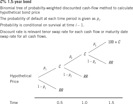
The survival curve is used to price the bond in line with a binomial tree model. This is shown in FIGURE 5.2, where we see that the bond's cash flow of coupon and principal follows a binomial path of payment if no default or payment of recovery amount RR in event of default. Each cash flow is discounted at the swap rate relevant to that term; the discounting is weighted according to the relevant term default probability. The sum of these probability-weighted discounted cash flows is the bond's hypothetical price. It represents the price of the CDS if it traded as a bond, in effect the price of a credit-linked note or funded CDS. For simplicity, the cash flow at each payment date can be discounted at a single market rate such as the swap rate or Libor rate as well. The aggregate of these cash flows, the hypothetical bond price, will differ from the observed market price.

The adjusted CDS spread is the spread above (or below) the swap curve that equates the bond's observed market price to its hypothetical price calculated above.

The adjusted CDS spread can be viewed as the Z-spread of the bond at its hypothetical price. Comparing it to the actual Z-spread, then, gives us a like-for-like comparison and a more robust measure of the basis.

FIGURE 5.2 Calculating the bond hypothetical price using implied default probabilities

In other words, we produce an adjusted Z-spread based on CDS prices, and compare it to the Z-spread of the bond at its actual market price. We have still compared the synthetic asset price to the cash asset price, as given originally in equation (3.1) in Chapter 3, but the comparison is now a logical one.

The alternative approach we suggested earlier of adjusting a bond spread into an equivalent CDS spread can also be followed, but suffers from a paucity of observable market data. We would need a sufficient number of bonds with maturities from the short to the long end of the curve, and this is available only from large issuers with continuous programs, such as Ford. On the other hand, as we noted earlier, the CDS market can be used to plot a credit curve for many more reference names out to the 20-year end of the curve or even beyond.

FIGURE 5.3 Illustrating the hypothetical bond price calculation based on CDS-implied default probability

Illustration

We illustrate the technique with an example using a hypothetical corporate bond, the ABC PLC 6% of 2008. This is shown in FIGURE 5.3. We set it so that the ABC PLC bond has exactly 3 years to maturity, and we discount the cash flows using only the 3-year rate, rather than each cash flow at its own specific term discount rate. This is just to simplify the calculation. If we have fractions in the remaining time to maturity, we use the exact time period (in years) to adjust the default probabilities.

The market price of the bond is $102.47. The hypothetical price is $101.87. The Z-spread of the bond at its market price is 14 basis points. To calculate the adjusted Z-spread, we apply the process we described earlier in this chapter; this gives us an adjusted Z-spread, or hypothetical price Z-spread, of 19.9 basis points. This is near to the CDS spread of 21 basis points.

The adjusted basis is therefore

which is 19.9 – 14, or 5.9 basis points. Compare this to the conventional basis, which is

which is 21 – 23.12, or −2.12 basis points.

So the true basis is, in this example, not negative but positive. Further analysis of the kind we have undertaken would have argued against a basis trade that might have looked attractive due to the negative basis indicating potential value.

Market Observation

The foregoing highlights some of the issues involved in measuring the basis. Irrespective of the calculation method employed, the one certainty is that corporate names in cash and synthetic markets do trade out of line; the basis is driven across positive and negative ranges due to the impact of a diverse range of technical, structural, and market factors (see Chapter 3). Of course, any basis value that is not zero implies potential value in arbitrage trades in that reference name, be it buying or selling the basis.

FIGURE 5.4 Selected telecoms corporate name, cash-CDS basis, 2003-2005

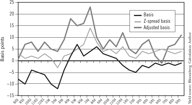
The conventional situation is a positive basis, as a negative basis implies a risk-free arbitrage profit is available. Market observation suggests that a negative basis is more common than might be expected, however. FIGURE 5.4 shows the basis—measured in each of the three ways we have highlighted—for a selected corporate name in the telecoms sector for the period August 2003 to September 2005. There is occasional relatively wide divergence between the measures, but all measures show the move from positive to negative territory and then back again.

Summary

The high level of liquidity now available in synthetic credit markets, which now encompass structured finance securities as well corporate names, has resulted in basis trading's becoming an important sector in relative value trading. Because value in the cash market can be measured in a number of ways as a spread to Libor, a key issue when calculating the basis is which Libor spread measure to use. This is not an issue for the CDS leg of the equation, as there is only one, unambiguous value for a CDS.

The most common spread measure is the asset-swap spread. As a par product, this becomes an inaccurate measure of credit risk if the bond itself is trading away from par. The Z-spread, while a more appropriate measure of value than the ASW spread, also suffers from not incorporating any element of default probability in its calculation.

We observed that the basis is driven by coupon and convexity issues, which we formalized in a relationship among the spread of the bond, its coupon, and the respective durations of the bond and CDS. We determined that the adjusted Z-spread was the most effective measure of the cash market to use when measuring the basis. The approach to calculate this creates a hypothetical bond price from default-probability-weighted discounted cash flows. Using this measure enables us to compare like-for-like, and so arrive at a more logical value for the basis. This should enable investors to better analyze potential value in relative value trades.

References

Choudhry, M. 2004. Structured credit products: Credit derivatives and synthetic securitisation. Singapore: John Wiley & Sons.