CHAPTFR 2

Bond Spreads and Relative Value

The credit default swap (CDS) basis is an important measure of relative value in the credit markets. Before considering the basis itself, we must familiarize ourselves with some basic concepts of bond spreads. An understanding of these is important when we consider the CDS basis later. In this chapter, we also introduce the theoretical concept of the cash market-synthetic market basis, when we consider (and then discard) the asset-swap pricing methodology for CDS contracts.

Bond Spreads

Investors measure the perceived market value, or relative value, of a corporate bond by measuring its yield spread relative to a designated benchmark. This is the spread over the benchmark that gives the yield of the corporate bond. A key measure of relative value of a corporate bond is its swap spread. This is the basis-point spread over the interest-rate swap curve, and is a measure of the credit risk of the bond. In its simplest form, the swap spread can be measured as the difference between the yield-to-maturity of the bond and the interest rate given by a straight-line interpolation of the swap curve. In practice, traders use the asset-swap spread and the Z-spread as the main measures of relative value. The government bond spread is also used. In addition, now that the market in synthetic corporate credit is well established, using credit derivatives and CDS, investors consider the cash-CDS spread as well, which is the basis, and which we consider in greater detail later.

The spread that is selected is an indication of the relative value of the bond, and a measure of its credit risk. The greater the perceived risk, the greater the spread should be. This is best illustrated by the credit structure of interest rates, which will (generally) show AAA- and AA-rated bonds trading at the lowest spreads, and BBB-, BB-, and lower-rated bonds trading at the highest spreads. Bond spreads are the most commonly used indication of the risk-return profile of a bond.

In this section, we consider the Treasury spread, asset-swap spread, Z-spread and basis.

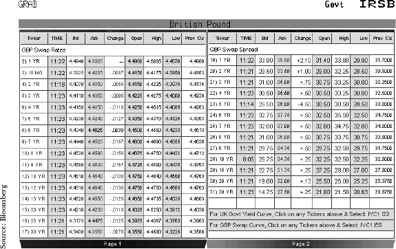
Swap Spread and Treasury Spread

A bond's swap spread is a measure of the credit risk of that bond, relative to the interest-rate swaps market. Because the swaps market is traded by banks, this risk is effectively the interbank market, so the credit risk of the bond over and above bank risk is given by its spread over swaps. This is a simple calculation to make, and is simply the yield of the bond minus the swap rate for the appropriate maturity swap. FIGURE 2.1 shows Bloomberg page IRSB for pounds sterling as of September 22, 2005. This shows the GBP swap curve on the left-hand side. The right-hand side of the screen shows the swap rates' spread over U.K. gilts. It is the spread over these swap rates that would provide the simplest relative value measure for corporate bonds denominated in GBP. If the bond has an odd maturity, say 5.5 years, we would interpolate between the 5-year and 6-year swap rates.

The spread over swaps is sometimes called the I-spread. It has a simple relationship to swaps and Treasury yields, shown here in the equation for corporate bond yield

FIGURE 2.1 Bloomberg page IRSB for pounds sterling, showing GBP swap rates and swap spread over U.K. gilts, September 22, 2005

where

In other words, the swap rate itself is given by T + S.

The I-spread is sometimes used to compare a cash bond with its equivalent CDS price, but for straightforward relative value analysis, is usually dropped in favor of the asset-swap spread, which we look at later in this section.

Of course the basic relative value measure is the Treasury spread, or government bond spread. This is simply the spread of the bond yield over the yield of the appropriate government bond. Again, an interpolated yield may need to be used to obtain the right Treasury rate to use. The bond spread is given by

Using an interpolated yield is not strictly accurate because yield curves are smooth in shape, and so straight-line interpolation will produce slight errors. The method is still commonly used, though.

Asset-Swap Spread

An asset swap is a package that combines an interest-rate swap with a cash bond, the effect of the combined package being to transform the interest-rate basis of the bond. Typically, a fixed-rate bond will be combined with an interest-rate swap in which the bondholder pays fixed coupon and receives floating coupon. The floating coupon will be a spread over Libor (see Choudhry et al. [2001]). This spread is the asset-swap spread, and is a function of the credit risk of the bond over and above interbank credit risk.¹ Asset swaps may be transacted at par or at the bond's market price, usually par. This means that the asset-swap value is made up of the difference between the bond's market price and par, as well as the difference between the bond coupon and the swap fixed rate.

The zero-coupon curve is used in the asset-swap valuation. This curve is derived from the swap curve, so it is the implied zero-coupon curve. The asset-swap spread is the spread that equates the difference between the present value of the bond's cash flows, calculated using the swap zero rates, and the market price of the bond. This spread is a function of the bond's market price and yield, its cash flows, and the implied zero-coupon interest rates.²

FIGURE 2.2 Bloomberg page ASW for GKN bond, August 10, 2005

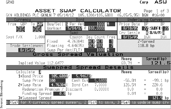
FIGURE 2.2 shows the Bloomberg screen ASW for a GBP-denominated bond, GKN Holdings 7% 2012, as of August 10, 2005. We see that the asset-swap spread is 121.5 basis points. This is the spread over Libor that will be received if the bond is purchased in an asset-swap package. In essence, the asset-swap spread measures a difference between the market price of the bond and the value of the bond when cash flows have been valued using zero-coupon rates. The asset-swap spread can therefore be regarded as the coupon of an annuity in the swap market that equals this difference.

Z-Spread

The conventional approach for analyzing an asset swap uses the bond's yield-to-maturity (YTM) in calculating the spread. The assumptions implicit in the YTM calculation (see Chapter 6 of Choudhry et al. [2001]) make this spread problematic for relative analysis, so market practitioners use what is termed the Z-spread instead. The Z-spread uses the zero-coupon yield curve to calculate spread, so is a more realistic, and effective, spread to use. The zero-coupon curve used in the calculation is derived from the interest-rate swap curve.

Put simply, the Z-spread is the basis-point spread that would need to be added to the implied spot yield curve such that the discounted cash flows of a bond are equal to its present value (its current market price). Each bond cash flow is discounted by the relevant spot rate for its maturity term. How does this differ from the conventional asset-swap spread? Essentially, in its use of zero-coupon rates when assigning a value to a bond. Each cash flow is discounted using its own particular zero-coupon rate. The price of a bond at any time can be taken to be the market's value of the bond's cash flows. Using the Z-spread, we can quantify what the swap market thinks of this value—that is, by how much the conventional spread differs from the Z-spread. Both spreads can be viewed as the coupon of a swap market annuity of equivalent credit risk of the bond being valued.

In practice, the Z-spread, especially for shorter-dated bonds and for better credit-quality bonds, does not differ greatly from the conventional asset-swap spread. The Z-spread is usually the higher spread of the two, following the logic of spot rates, but not always. If it differs greatly, then the bond can be considered to be mispriced.

FIGURE 2.3 is the Bloomberg screen YAS for the same bond shown in Figure 2.2, as of the same date. It shows a number of spreads for the bond. The main spread of 151.00 basis points (bps) is the spread over the government yield curve. This is an interpolated spread, as can be seen lower down the screen, with the appropriate benchmark bond identified. We see that the asset-swap spread is 121.6 bps, while the Z-spread is 118.8 bps. When undertaking relative value analysis, for instance if making comparisons against cash funding rates or the same company name CDS, it is this lower spread that should be used.³

FIGURE 2.3 Bloomberg page YAS for GKN bond, August 10, 2005

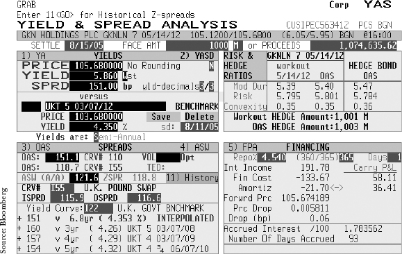
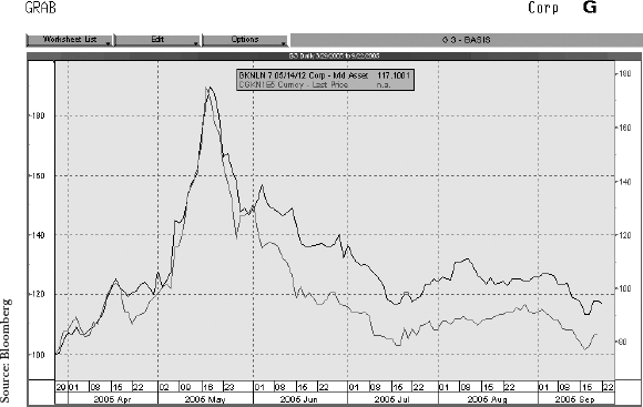
FIGURE 2.4 Bloomberg page YAS for GKN bond, August 10, 2005, showing 7-spread history

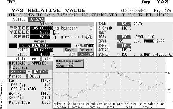
The same screen can be used to check spread history. This is shown in FIGURE 2.4, the Z-spread graph for the GKN bond for the 6 months prior to our calculation date.

The Z-spread is closely related to the bond price, as shown by

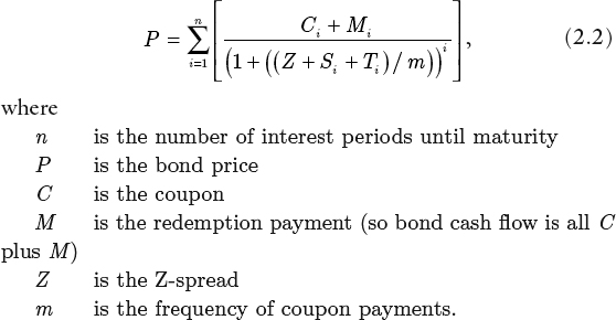
In effect, this is the standard bond price equation with the discount rate adjusted by whatever the Z-spread is; it is an iterative calculation. The appropriate maturity swap rate is used, which is the essential difference between the I-spread and the Z-spread. This is deemed to be more accurate, because the entire swap curve is taken into account rather than just one point on it. In practice, though, as we have seen in the example above, there is often little difference between the two spreads.

To reiterate, then, using the correct Z-spread, the sum of the bond's discounted cash flows will be equal to the current price of the bond.

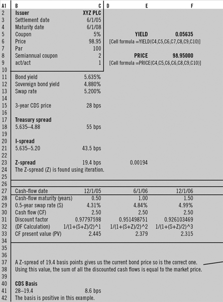
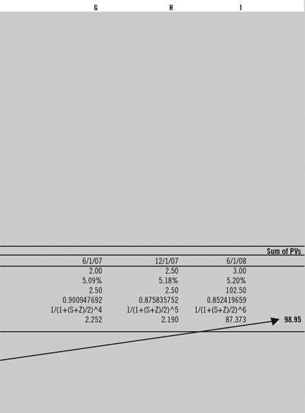
We illustrate the Z-spread calculation in FIGURE 2.5 (see pages 46 and 47). This is done using a hypothetical bond, the XYZ PLC 5% of June 2008, a 3-year bond at the time of the calculation. Market rates for swaps, Treasury, and CDS are also shown. We require the spread over the swaps curve that equates the present values of the cash flows to the current market price. The cash flows are discounted using the appropriate swap rate for each cash-flow maturity. With a bond yield of 5.635%, we see that the I-spread is 43.5 basis points, while the Z-spread is 19.4 basis points. In practice, the difference between these two spreads is rarely this large.

For readers' benefit, we also show the Excel formula in Figure 2.5. This shows how the Z-spread is calculated; for ease of illustration, we have assumed that the calculation takes place for value on a coupon date, so that we have precisely an even period to maturity.

The Asset-Swap CDS Price

Credit default swaps provide an efficient means of pricing pure credit, and by definition are a measure of the credit risk of a specific reference entity or reference asset. Asset swaps are well established in the market, and are used both to transform the cash-flow structure of a corporate bond and to hedge against interest-rate risk of a holding in such a bond. Because asset swaps are priced at a spread over Libor, with Libor representing interbank risk, the asset-swap spread represents in theory the credit risk of the asset-swap name. By the same token, using the no-arbitrage principle, it can be shown that the price of a credit default swap for a specific reference name should equate the asset-swap spread for the same name. However a number of factors, both structural and operational, combine to make credit default swaps trade at a different level to asset swaps. These factors are investigated in greater detail in Chapter 3. This difference in spread is the credit default swap basis, and can be either positive (the credit default swap trading above the asset-swap level) or negative (trading below the asset-swap level).

Asset-Swap Pricing

At the inception of the market, credit derivatives were valued using the asset-swap pricing technique. We will explain shortly why this approach is no longer used. Let us first consider, however, the theoretical reason why they should be priced using this approach.

A par asset swap typically combines the sale of an asset such as a fixed-rate corporate bond to a counterparty, at par and with no interest accrued, with an interest-rate swap. The coupon on the bond is paid in return for Libor, plus a spread if necessary. This spread is the asset-swap spread and is the price of the asset swap. In effect, the asset swap allows market participants that pay Libor-based funding to receive the asset-swap spread. This spread is a function of the credit risk of the underlying bond asset, which is why it could be viewed as equivalent to the price payable on a credit default swap written on that asset.

FIGURE 2.5 Calculating the Z-spread, hypothetical 5% 2008 hond issued by XYZ PLC

The generic pricing is given by

The asset spread over the benchmark is simply the bond (asset) redemption yield over that of the government benchmark. The interest-rate swap spread reflects the cost involved in converting fixed-coupon benchmark bonds into a floating-rate coupon during the life of the asset (or default swap), and is based on the swap rate for that maturity.

The theoretical basis for deriving a default swap price from the asset-swap rate can be illustrated by looking at a basis-type trade involving a cash market reference asset (bond) and a default swap written on this bond. This is similar in concept to the risk-neutral, or no-arbitrage, concept used in derivatives pricing. The theoretical trade involves:

• A long position in the cash market floating-rate note (FRN) priced at par, and which pays a coupon of Libor + X basis points
• A long position (bought protection) in a default swap written on the same FRN, of identical term-to-maturity and at a cost of Y basis points

The buyer of the bond is able to fund the position at Libor. In other words, the bondholder has the following net cash flow:

or X − Y basis points.

In the event of default, the bond is delivered to the protection seller in return for payment of par, enabling the bondholder to close out the funding position. During the term of the trade, the bondholder has earned X − Y basis points while assuming no credit risk. For the trade to meet the no-arbitrage condition, we must have X = Y. If X ≠ Y, the investor would be able to establish the position and generate a risk-free profit.

This is a logically tenable argument as well as a reasonable assumption. The default risk of the cash bondholder is identical in theory to that of the default seller. In the next section, we illustrate an asset-swap pricing example, before looking at why in practice there exist differences in pricing between default swaps and cash market reference assets.

Asset-Swap Pricing Example

XYZ PLC is a Baa2-rated corporate. The 7-year asset swap for this entity is currently trading at 93 basis points; the underlying 7-year bond is hedged by an interest-rate swap with an Aa2-rated bank. The risk-free rate for floating-rate bonds is Libid minus 12.5 basis points (assume the bid-offer spread is 6 basis points). This suggests that the credit spread for XYZ PLC is 111.5 basis points. The credit spread is the return required by an investor for holding the credit of XYZ PLC. The protection seller is conceptually long the asset, and so would short the asset to hedge its position. This is illustrated in FIGURE 2.6. The price charged for the default swap is the price of shorting the asset, which works out as 111.5 basis points each year.

Therefore, we can price a credit default written on XYZ PLC as the present value of 111.5 basis points for 7 years, discounted at the interest-rate swap rate of 5.875%. This computes to a credit swap price of 6.25%.

FIGURE 2.6 Credit default swap and asset-swap hedge

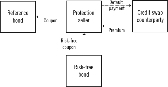
Reference	XYZ PLC
Term	7 years
Interest-rate swap rate	5.875%
Asset swap	Libor plus 93 bps
Default swap pricing:
Benchmark rate	Libid minus 12.5 bps
Margin	6 bps
Credit default swap	111.5 bps
Default swap price	6.252%

Pricing Differentials

A number of factors observed in the market serve to make the price of credit risk that has been established synthetically using default swaps to differ from its price as traded in the cash market. In fact, identifying (or predicting) such differences gives rise to arbitrage opportunities that may be exploited by basis trading in the cash and derivative markets.⁴ These factors include the following:

Bond identity: the bondholder is aware of the exact issue that he is holding in the event of default; however, default swap sellers may receive potentially any bond from a basket of deliverable instruments that rank pari passu with the cash asset; this is the delivery option afforded the long swap holder.

The borrowing rate for a cash bond in the repo market may differ from Libor if the bond is to any extent special; this does not impact the default swap price, which is fixed at inception.

Certain bonds rated AAA (such as U.S. agency securities) sometimes trade below Libor in the asset-swap market; however, a bank writing protection on such a bond will expect a premium (positive spread over Libor) for selling protection on the bond.

Depending on the precise reference credit, the default swap may be more liquid than the cash bond, resulting in a lower default swap price, or less liquid than the bond, resulting in a higher price.

Credit default swaps may be required to pay out on credit events that are technical defaults, and not the full default that impacts a cash bondholder; protection sellers may demand a premium for this additional risk.

The credit default swap buyer is exposed to counterparty risk during the term of the trade, unlike the cash bondholder.

For these and other reasons, the credit default swap price differs from the cash market price for the same asset. Therefore, banks are increasingly turning to credit pricing models, based on the same models used to price interest-rate derivatives, when pricing credit derivatives.

Illustration Using the BLOOMBERG PROFESSIONAL® Service

Observations from the market show the difference in price between asset swaps on a bond and a credit default swap written on that bond, reflecting the factors stated in the previous section. We illustrate this now using a euro-denominated corporate bond.

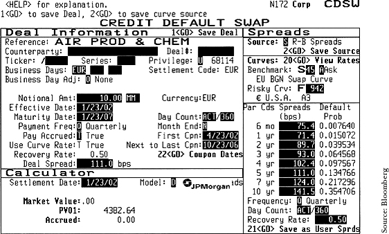
FIGURE 2.7 Bloomberg page DES for Air Products & Chemicals bond

The bond is the Air Products & Chemicals 6½% bond due July 2007. This bond is rated A3/A as shown in FIGURE 2.7, the description page from the Bloomberg. The asset-swap price for that specific bond to its term to maturity as of January 18, 2002, was 41.6 basis points. This is shown in FIGURE 2.8. The relevant swap curve used as the pricing reference is indicated on the screen as curve 45, which is the Bloomberg reference number for the euro swap curve and is shown in FIGURE 2.9.

We now consider the credit default swap page on the Bloomberg for the same bond, which is shown in FIGURE 2.10. For the similar maturity range, the credit default swap price would be approximately 115 basis points. This differs significantly from the asset-swap price.

From the screen, we can see that the benchmark curve is the same as that used in the calculation shown in Figure 2.9. The corporate curve used as the pricing reference, however, is indicated as the euro-denominated U.S.-issuer A3 curve, and this is shown in FIGURE 2.11. This is page CURV on the Bloomberg, and is the fair value corporate credit curve constructed from a basket of A3 credits. On the following pages of the same screen, the user can view the list of bonds that are used to construct the curve. For comparison, we also show the Bank A3-rated corporate credit yield curve in FIGURE 2.12.

FIGURE 2.8 Asset-swap calculator on Bloomberg page ASW, January 18, 2002

FIGURE 2.9 Euro swap curve on Bloomberg page SWDF as of January 18, 2002

FIGURE 2.10 Default swap page CDSW for Air Products & Chemicals bond, January 18, 2002

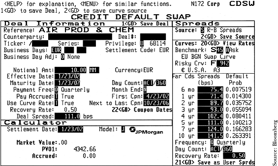
FIGURE 2.11 Fair market curve, euro A3 sector

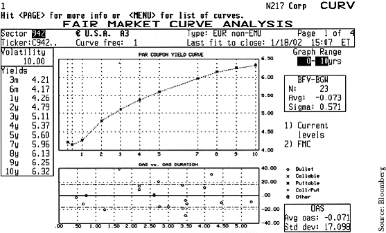
FIGURE 2.12 Fair market curve, euro Banks A3 sector

Prices observed in the market will invariably show this pattern of difference between the asset-swap price and the credit default swap price. The page CDSW on the Bloomberg uses the generic risky curve to calculate the default swap price, and adds the credit spread to the interest-rate swap curve. However, the ASW page is the specific asset-swap rate for that particular bond, to the bond's term to maturity; this is another reason why the prices of the two instruments will differ significantly.

On the Bloomberg, the user can select either the JPMorgan credit default swap pricing model or a generic discounted credit spreads model. These are indicated by “J” or “D” in the box marked “Model” on the CDSW page. FIGURE 2.13 shows this page with the generic model selected. Although there is no difference in the swap prices, the default probabilities, as expected, have changed under this setting.

FIGURE 2.13 CDSW page with discounted spreads model selected

Our example illustrates the difference in swap price that we discussed earlier, and can be observed for any number of corporate credits across sectors. This suggests that middle-office staff and risk managers that use the asset-swap technique to independently value default swap books are at risk of obtaining values that differ from those in the market. This is an important issue for credit derivative market-making banks.

Cash-CDS Basis

We see then that the basis is the CDS spread minus the ASW spread. Alternatively, it can be the CDS spread minus the Z-spread. So the basis is given by

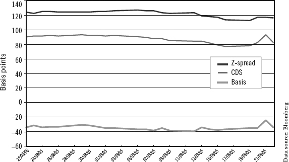
FIGURE 2.14 Bloomberg graph using screen G <Go>, plot of asset-swap spread and CDS price for GKN bond, April–September 2005

where D is the CDS price. Where D – CashSpread > 0, it is a positive basis; the opposite is a negative basis.

FIGURE 2.14 shows page G <Go> on the Bloomberg, set up to show the Z-spread and CDS price history for the GKN 2012 bond for the period March–September 2005. We can select the “Table” option to obtain the actual values, which can then be used to plot the basis. This is shown in FIGURE 2.15, for the period August 22 to September 22, 2005. Notice how the basis was always negative during August–September; we see from Figure 2.14 that earlier in the year, the basis had briefly been positive. Changes in the basis give rise to arbitrage opportunities between the cash and synthetic markets. This is discussed in greater detail in Choudhry (2004b).

A wide range of factors drive the basis; these factors are described in detail in Chapter 3. The existence of a non–zero basis has implications for investment strategy. For instance, when the basis is negative, investors may prefer to hold the cash bond; whereas, if—for liquidity, supply, or other reasons—the basis is positive, the investor may wish to hold the asset synthetically, by selling protection using a credit default swap. Another approach is to arbitrage between the cash and synthetic markets, in the case of a negative basis by buying the cash bond and shorting it synthetically by buying protection in the CDS market. Investors have a range of spreads to use when performing their relative value analysis.

FIGURE 2.15 GKN bond, CDS basis during August–September 2005

References

Choudhry, M., D. Joannas, R. Pienaar, and R. Pereira. 2001. Capital market instruments: Analysis and valuation. Upper Saddle River, NJ: FT Prentice Hall.

Choudhry, M. 2004a. Structured credit products: Credit derivatives and synthetic securitisation. Singapore: John Wiley & Sons.

——. 2004b. The credit default swap basis: Analysing the relationship between cash and synthetic markets. Journal of Derivatives Use, Trading and Regulation 10 (1) (June): 9–26.