Chapter 11. Processing and partitioning tabular models
After you create a tabular model, you should deploy it in a production environment. This requires you to plan how you will partition and process the data. This chapter has extensive coverage of these topics, with particular attention given to design considerations that give you the knowledge to make the right decisions based on your specific requirements. You will also find step-by-step guides to introduce you to the use of certain functions that you will see for the first time in this chapter.
![]() What’s new in SSAS 2016
What’s new in SSAS 2016
The concepts behind process and partitioning are the same as in previous versions, but SSAS 2016 has new scripts, libraries, and tools to manage processing, deployment, and partitioning for models with compatibility level 1200 or higher.
Automating deployment to a production server
You can deploy a tabular model to a production server in the following ways:
![]() By deploying it directly from SQL Server Data Tools (SSDT) This deploys the model according to the deployment server configuration of your project. Visual Studio 2015 configurations support tabular projects (which were not supported in previous versions of Visual Studio). You can create different configurations with different deployment server properties such as the server and database name. For example, you can create different configurations for development, a user acceptance test, and the production environments.
By deploying it directly from SQL Server Data Tools (SSDT) This deploys the model according to the deployment server configuration of your project. Visual Studio 2015 configurations support tabular projects (which were not supported in previous versions of Visual Studio). You can create different configurations with different deployment server properties such as the server and database name. For example, you can create different configurations for development, a user acceptance test, and the production environments.
![]() By using the Analysis Services Deployment Wizard This can generate a deployment script that you can forward to an administrator. The administrator can then execute the script directly in SSMS by using the
By using the Analysis Services Deployment Wizard This can generate a deployment script that you can forward to an administrator. The administrator can then execute the script directly in SSMS by using the ASCmd cmdlet in PowerShell (https://msdn.microsoft.com/en-us/library/hh479579.aspx) or by scheduling it in SQL Server Agent, provided he or she has the required administrative rights. For further information about the wizard, refer to the documentation available on MSDN at https://msdn.microsoft.com/en-us/library/ms176121(v=sql.130).aspx.
![]() By using the Synchronize Database Wizard or by executing the script that this wizard can generate This wizard copies the contents of a database from a source server that you select to a target server. The server on which the wizard has been selected is the target server and will receive the
By using the Synchronize Database Wizard or by executing the script that this wizard can generate This wizard copies the contents of a database from a source server that you select to a target server. The server on which the wizard has been selected is the target server and will receive the Synchronize command in a script. This option can be useful to move a database that is deployed on a development or test server to a production server. It is also useful when you want to duplicate the tabular database in a server farm that is part of a scale-out architecture. You can find more information about synchronizing databases in Analysis Services at https://msdn.microsoft.com/en-us/library/ms174928(v=sql.130).aspx.
You can also automate the deployment from SSDT by using a custom post-build task that performs the deployment by using the MSBuild tool. Follow the instructions at https://blogs.msdn.microsoft.com/cathyk/2011/08/10/deploying-tabular-projects-using-a-custom-msbuild-task/.
Table partitioning
An important design decision in a tabular model using in-memory mode is the partitioning strategy. Every table in Tabular can be partitioned, and the reason for partitioning is related exclusively to table processing. As you will see in Chapter 12, “Inside VertiPaq,” partitions do not give query performance benefits in Tabular. They are useful only to reduce the time required to refresh data because you can update just the parts of a table that have been updated since the previous refresh. In this section, you learn when and how to define a partitioning strategy for your tabular model.
Defining a partitioning strategy
Every table in Tabular has one or more partitions. Every partition defines a set of rows that are read from the source table. Every partition can be processed independently and in parallel with others, so you can use partitions to accelerate the processing of a single table. Parallel processing of partitions was not possible in previous versions of Analysis Services, but it is available with Analysis Services 2016 for any compatibility level (including the 110x ones).
You define partitions related to the source table, but from the Tabular point of view, every table is made of several columns, and every column is a different object. Some columns are calculated and based on the data of other columns belonging to the same or different tables. The engine knows the dependencies of each calculated column and calculated table. When you process a partition of a table, every dependent calculated table must be completely recalculated. Moreover, every calculated column in the same or other tables must be completely recalculated for the entire table to which it belongs.
Calculated tables cannot have more than one partition. Even if they are calculated according to the dependency order that is automatically recognized by the engine, the evaluation and compression of the calculated table could be faster than the time required to evaluate a correspondent number of calculated columns in a table that has the same number of rows.
Finally, other indexing structures exist for storing column dictionaries and relationships between tables. These structures are not partitioned and require recalculation for the whole table to which they belong if a column on which they depend has been refreshed (even if only for one partition).
![]() Note
Note
In a multidimensional model, only measure groups can be partitioned, and you cannot create partitions over dimensions. When a measure group partition is processed, all the aggregations must be refreshed, but only for the partition. However, when a dimension is refreshed, it might invalidate aggregations of a related measure group. Dependencies between partitions and related structures, such as indexes and aggregations, in a multidimensional model might seem familiar. In reality, however, they are completely different, and the partitioning strategy can be very different between multidimensional and tabular models that use the same data source. For example, processing a table in Tabular that is a dimension in a star schema does not require you to rebuild indexes and aggregations on the measure group that corresponds to the fact table in the same star schema. Relationships and calculated columns are dependent structures that must be refreshed in Tabular, but their impact is usually lower than that incurred in a multidimensional model.
The following are reasons for creating more partitions for a table:
![]() Reducing processing time When the time required for processing the whole table is too long for the available processing window, you can obtain significant reduction by processing only the partitions that contain new or modified data.
Reducing processing time When the time required for processing the whole table is too long for the available processing window, you can obtain significant reduction by processing only the partitions that contain new or modified data.
![]() Easily removing data from a table You can easily remove a partition from a table. This can be useful when you want to keep the last n months in your tabular model. By using monthly partitions, every time you add a new month, you create a new partition, removing the older month by deleting the corresponding partition.
Easily removing data from a table You can easily remove a partition from a table. This can be useful when you want to keep the last n months in your tabular model. By using monthly partitions, every time you add a new month, you create a new partition, removing the older month by deleting the corresponding partition.
![]() Consolidating data from different source tables Your source data is divided into several tables, and you want to see all the data in a single table in Tabular. For example, suppose you have a different physical table in the source database for each year of your orders. In that case, you could have one partition in Tabular for every table in your data source.
Consolidating data from different source tables Your source data is divided into several tables, and you want to see all the data in a single table in Tabular. For example, suppose you have a different physical table in the source database for each year of your orders. In that case, you could have one partition in Tabular for every table in your data source.
The most common reason is the need to reduce processing time. Suppose you can identify only the rows that were added to the source table since the last refresh. In that case, you might use the Process Add operation. This operation reads from the data source only the rows to add, implicitly creates a new partition, and merges it with an existing one, as you will see later in this chapter in the section “Managing partitions for a table.” The processing time is faster because it only reads the new rows from the data source. However, Process Add can be used only when the existing data in the partition will be never modified. If you know that a row that was already loaded has changed in the data source, you should reprocess the corresponding partition containing that row.
![]() Note
Note
An alternative approach to handling data change is to use Process Add to insert a compensating transaction. This is very common in a multidimensional model. However, because a table can be queried in Tabular without aggregating data, this approach would result in showing all the compensating transactions to the end user.
Partitions do not give you a benefit at query time, and a very high number of partitions (100 or more) can be counterproductive because all the partitions are considered during queries. VertiPaq cannot ignore a partition based on its metadata, as Analysis Services does with a multidimensional model that contains partitions with a slice definition. A partition should merely define a set of data that can be easily refreshed or removed from a table in a tabular model.
You can merge partitions—for example, by merging all the days into one month or all the months into one year. Merging partitions does not process data and therefore does not require you to access the data source. This can be important when data access is an expensive operation that occupies a larger part of the process operation. Other activities, such as refreshing internal structures, might still be required in a merge, but they are done without accessing the data sources.
Finally, carefully consider the cost of refreshing indexing structures after you process one or more partitions. (See the “Process Recalc” section later in this chapter). With complex models, this could be an important part of the process, and you must lower the object dependencies to reduce the time required to execute a Process Recalc operation. Moreover, if you remove partitions or data changes in existing partitions that are refreshed, you must plan a Process Defrag operation to optimize the table dictionary, reduce memory consumption, and improve query performance. Thus, implementing a partitioning strategy requires you to make a plan for maintenance operations. This maintenance is not required when you use the Process Full operation on a table because this operation completely rebuilds the table.
![]() Important
Important
Do not underestimate the importance of Process Defrag if you have a partitioned table where you never run a full process over the entire table. Over time, the dictionary might continue to grow with values that are never used. When this happens, you have two undesirable side effects: The dictionary becomes unwieldy and the compression decreases in efficiency because the index to the dictionary might require more bits. This can result in higher memory pressure and lower performance. A periodic Process Defrag might be very useful in these scenarios.
Defining partitions for a table in a tabular model
After you define your partition strategy, the first place in which you can create table partitions is the project of the tabular model. This option is useful mainly if you have a fixed number of partitions—because, for example, data comes from different tables or the partitioning key is not based on time. If you have a more dynamic structure of partitions, you can change them by using SSMS or scripts, as you will see in the following sections. In this section, you learn how to create partitions by using SSDT. Follow these steps:
1. Open the Table menu and choose Partitions to open the Partition Manager dialog box, shown in Figure 11-1. Here, you can edit the partitions for a table. In this example, the Customer table has just one partition (Customer) with 18,484 rows.

2. The Table Preview and Query Editor buttons enable you to choose the content shown in the Details area below the Source Name drop-down list. Figure 11-1 shows Table Preview mode, which displays the columns and rows that can be read from the table selected in the Source Name drop-down list (in this case, Analytics.Customer). Select values for one column to filter data in the table preview and implicitly define a query that applies the same filter when processing the partition. Figure 11-2 shows how to select just a few values for the Education column.

This is just an example to show you the Partition Manager user interface. It is not a best practice. This is because you should not partition columns that will change over time. This is not the case with the Education column because a customer might in fact change her education over time, changing the partition to which she belongs. A better partitioning column for Customer could be Country of Birth because it cannot change over time. However, the sample database does not have such a column.
3. Click the Query Editor button to view and edit the query in the Customer partition. The query that is generated depends on the sequence of operations you perform through the user interface. For example, if you start from the default setting (all items selected) and clear the Partial College, Partial High School, and (blanks) items, you obtain the query shown in Figure 11-3. This includes all future values, excluding those you cleared in the list.

Figure 11-3 The Partition query obtained by clearing values in the list, which contains a NOT in the WHERE condition.
4. Clear the Select All check box and then manually select the Bachelor, Graduate Degree, and High School columns to obtain a SQL statement that includes only the values you explicitly selected in the list, as shown in Figure 11-4.

Figure 11-4 The Partition query obtained by clearing the Select All check box and selecting values in the list. The query includes only the selected items in the WHERE condition.
5. Edit the SQL statement manually by creating more complex conditions. Note, however, that when you do, you can no longer use Table Preview mode without losing your query. The message shown in Figure 11-5 warns you of this when you click the Table Preview button.

Figure 11-5 Showing how the manual changes to the SQL statement are lost by going back to the Table Preview mode.
6. After you create a new partition or copy an existing one, change the filters in Table Preview mode or in the SQL statement in the Query Editor to avoid the same data being loaded into more than one partition. You do not get any warning at design time about the potential for data duplication. The process operation will fail only if a column that is defined as a row identifier is duplicated.
7. Often, you will need to select a large range of values for a partition. To do so, write a SQL statement that is like the one you see in the examples shown in Figure 11-6.
![]() Note
Note
After you modify the query’s SQL statement, you cannot switch back to the Table Preview mode. If you do, the SQL statement will be replaced by a standard SELECT statement applied to the table or view that is specified in the Source Name property.

Figure 11-6 How the Table Preview mode cannot be used when a partition is defined by using a SQL statement.
8.Check the SQL query performance and optimize it if necessary. Remember, one of the goals of creating a partition is to lessen the time required to process the data. Therefore, the SQL statement you write should also run quickly on the source database.
Managing partitions for a table
After you deploy a tabular model on Analysis Services, you can create, edit, merge, and remove partitions by directly modifying the published database without deploying a new version of the model itself. This section shows you how to manage partitions by using SSMS. Follow these steps:
1. Use SSMS to browse the tables available in a tabular model. Then right-click a table name and select Partitions in the context menu, as shown in Figure 11-7.

2. The Partitions dialog box opens. You can use this dialog box to manage the partitions of any table. Open the Table drop-down list and choose the table that contains the partition(s) you want to manage. As shown in Figure 11-8, a list of the partitions in that table appears, including the number of rows and the size and date of the last process for each partition.

3. Select the partition(s) you want to manage. Then click one of the buttons above the list of partitions. As shown in Figure 11-8, the buttons are as follows:
• New Click this button to create a new partition by using a default SQL statement that gets all the rows from the underlying table in the data source. You must edit this statement to avoid loading duplicated data in the tabular table.
• Edit Click this button to edit the selected partition. This button is enabled only when a single partition is selected.
• Delete Click this button to remove the selected partition(s).
• Copy Click this button to create a new partition using the same SQL statement of the selected partition. (You must edit the statement to avoid loading duplicated data in the tabular table.)
• Merge Click this button to merge two or more partitions. The first partition selected will be the destination of the merge operation. The other partition(s) selected will be removed after being merged into the first partition.
• Process Click this button to process the selected partition(s).
• Properties Click this button to view the properties of the selected partition. (This button is enabled only when a single partition is selected.)
Clicking the New, Edit, or Copy button displays the dialog box shown in Figure 11-9, except when you click New or Copy, the name of the dialog box changes to New Partition. Note that unlike with SSDT, there is no table preview or a query designer in SSMS for editing a partition.

4. Return to the Partitions dialog box shown in Figure 11-8 and select the following partitions: Sales 2007, Sales 2008, and Sales 2009. (To select all three, hold down the Ctrl key as you click each partition.) Then click the Merge button. The Merge Partition dialog box appears, as shown in Figure 11-10.

5. In the Source Partitions list, select the partitions you want to merge and click OK. The first partition you select will be the only partition that remains after the Merge operation. The other partitions selected in the Source Partitions list will be merged into the target partition and will be removed from the table (and deleted from disk) after the merge.
![]() Note
Note
For any operation you complete by using SSMS, you can generate a script (TMSL for compatibility level 1200, XMLA for compatibility levels 110x) that can be executed without any user interface. (Chapter 13, “Interfacing with Tabular,” covers this in more detail.) You can use such a script to schedule an operation or as a template for creating your own script, as you’ll learn in the “Processing automation” section later in this chapter.
Processing options
Regardless of whether you define partitions in your tabular model, when you deploy the model by using the in-memory mode, you should define how the data is refreshed from the data source. In this section, you learn how to define and implement a processing strategy for a tabular model.
Before describing the process operations, it is useful to quickly introduce the possible targets of a process. A tabular database contains one or more tables, and it might have relationships between tables. Each table has one or more partitions, which are populated with the data read from the data source, plus additional internal structures that are global to the table: calculated columns, column dictionaries, and attribute and user hierarchies. When you process an entire database, you process all the objects at any level, but you might control in more detail which objects you want to update. The type of objects that can be updated can be categorized in the following two groups:
![]() Raw data This is the contents of the columns read from the data source, including the column dictionaries.
Raw data This is the contents of the columns read from the data source, including the column dictionaries.
![]() Derived structures These are all the other objects computed by Analysis Services, including calculated columns, calculated tables, attribute and user hierarchies, and relationships.
Derived structures These are all the other objects computed by Analysis Services, including calculated columns, calculated tables, attribute and user hierarchies, and relationships.
In a tabular model, the derived structures should always be aligned to the raw data. Depending on the processing strategy, you might compute the derived structures multiple times. Therefore, a good strategy is to try to lower the time spent in redundant operations, ensuring that all the derived structures are updated to make the tabular model fully query-able. Chapter 12 discusses in detail what happens during processing, which will give you a better understanding of the implications of certain processing operations. We suggest that you read both this chapter and the one that follows before designing and implementing the partitioning scheme for a large tabular model.
A first consideration is that when you refresh data in a tabular model, you process one or more partitions. The process operation can be requested at the following three levels of granularity:
![]() Database The process operation can affect all the partitions of all the tables of the selected database.
Database The process operation can affect all the partitions of all the tables of the selected database.
![]() Table The process operation can affect all the partitions of the selected table.
Table The process operation can affect all the partitions of the selected table.
![]() Partition The process operation can only affect the selected partition.
Partition The process operation can only affect the selected partition.
![]() Note
Note
Certain process operations might have a side effect of rebuilding calculated columns, calculated tables, and internal structures in other tables of the same database.
You can execute a process operation by employing the user interface in SSMS or using other programming or scripting techniques discussed later in this chapter in the section “Processing automation.”
Available processing options
You have several processing options, and not all of them can be applied to all the granularity levels. Table 11-1 shows you the possible combinations, when using Available for operations that can also be used in the SSMS user interface and Not in UI for operations that can be executed only by using other programming or scripting techniques. The following sections describe what each operation does and what its side effects are.

Process Add
The Process Add operation adds new rows to a partition. It should be used only in a programmatic way. You should specify the query returning only new rows that must be added to the partition. After the rows resulting from the query are added to the partitions, only the dictionaries are incrementally updated in derived structures. All the other derived structures (calculated columns, calculated tables, hierarchies, and relationships) are automatically recalculated. The tabular model can be queried during and after a Process Add operation.
![]() Important
Important
Consider using Process Add only in a manually created script or in other programmatic ways. If you use Process Add directly in the SSMS user interface, it repeats the same query defined in the partition and adds all the resulting rows to the existing ones. If you want to avoid duplicated data, you should modify the partition so that its query will read only the new rows in subsequent executions.
Process Clear
Process Clear drops all the data in the selected object (Database, Table, or Partition). The affected objects are no longer query-able after this command.
Process Data
Process Data loads raw data in the selected object (Table or Partition), also updating the columns’ dictionaries, whereas derived structures are not updated. The affected objects are no longer query-able after this command. After Process Data, you should execute Process Recalc or Process Default to make the data query-able.
Process Default
Process Default performs the necessary operations to make the target object query-able (except when it is done at the partition level). If the database, table, or partition does not have data (that is, if it has just been deployed or cleared), it performs a Process Data operation first, but it does not perform Process Data again if it already has data. (This is true even if data in your data source has changed because Analysis Services has no way of knowing it has changed.) If dependent structures are not valid because a Process Data operation has been executed implicitly or before the Process Default operation, it applies a partial Process Recalc to only those invalid derived structures (calculated columns, calculated tables, hierarchies, and relationships). In other words, Process Default can be run on a table or partition, resulting in only Process Recalc on those specific objects, whereas Process Recalc can be run only on the database.
A Process Default operation completed at the database level is the only operation that guarantees that the table will be query-able after the operation. If you request Process Default at the table level, you should include all the tables in the same transaction. If you request Process Default for every table in separate transactions, be careful of the order of the tables because lookup tables should be updated after tables pointing to them.
A Process Default operation made at the partition level does a Process Data operation only if the partition is empty, but it does not refresh any dependent structure. In other words, executing Process Default on a partition corresponds to a conditional Process Data operation, which is executed only if the partition has never been processed. To make the table query-able, you must still run either Process Default at the database or table level or a Process Recalc operation. Using Process Recalc in the same transaction is a best practice.
Process Defrag
The Process Defrag operation rebuilds the column dictionaries without the need to access the data source to read the data again. It is exposed in the SSMS user interface for tables only. This operation is useful only when you remove partitions from your table or you refresh some partitions and, as a result, some values in columns are no longer used. These values are not removed from the dictionary, which will grow over time. If you execute a Process Data or a Process Full operation on the whole table (the latter is covered next), then Process Defrag is useless because these operations rebuild the dictionary.
![]() Tip
Tip
A common example is a table that has monthly partitions and keeps the last 36 months. Every time a new month is added, the oldest partition is removed. As a result, in the long term, the dictionary might contain values that will never be used. In these conditions, you might want to schedule a Process Defrag operation after one or more months have been added and removed. You can monitor the size of the dictionary by using VertiPaq Analyzer (http://www.sqlbi.com/tools/vertipaq-analyzer/), which is described in more detail in Chapter 12.
If you use Process Defrag at the database level, data for the unprocessed tables is also loaded. This does not happen when Process Defrag is run on a single table. If the table is unprocessed, it is kept as is.
Process Full
The Process Full operation at a database level is the easiest way to refresh all the tables and the related structures of a tabular model inside a transaction. This is so that the existing data is query-able during the whole process, and new data will not be visible until the process completes. All the existing data from all partitions are thrown away, every partition is loaded, all the tables are loaded, and then Process Recalc is executed over all the tables.
When Process Full is executed on a table, all the partitions of the table are thrown away, every partition is loaded, and a partial Process Recalc operation is applied to all the derived structures (calculated columns, calculated tables, hierarchies, and relationships). However, if a calculated column depends on a table that is unprocessed, the calculation is performed by considering the unprocessed table as an empty table. Only after the unprocessed table is populated will a new Process Recalc operation compute the calculated column again, this time with the correct value. A Process Full operation of the unprocessed table automatically refreshes this calculated column.
![]() Note
Note
The Process Recalc operation that is performed within a table’s Process Full operation will automatically refresh all the calculated columns in the other tables that depend on the table that has been processed. For this reason, Process Full over tables does not depend on the order in which it is executed in different transactions. This distinguishes it from the Process Defrag operation.
If Process Full is applied to a partition, the existing content of the partition is deleted, the partition is loaded, and a partial Process Recalc operation of the whole table is applied to all the derived structures (calculated columns, calculated tables, hierarchies, and relationships). If you run Process Full on multiple partitions in the same command, only one Process Recalc operation will be performed. If, however, Process Full commands are executed in separate commands, every partition’s Process Full will execute another Process Recalc over the same table. Therefore, it is better to include in one transaction multiple Process Full operations of different partitions of the same table. The only side effect to consider is that a larger transaction requires more memory on the server because data processed in a transaction is loaded twice in memory (the old version and the new one) at the same time until the process transaction ends. Insufficient memory can stop the process or slow it down due to paging activity, depending on the MemoryVertiPaqPagingPolicy server setting, as discussed in http://www.sqlbi.com/articles/memory-settings-in-tabular-instances-of-analysis-services.
Process Recalc
The Process Recalc operation can be requested only at the database level. It recalculates all the derived structures (calculated columns, calculated tables, hierarchies, and relationships) that must be refreshed because the underlying data in the partition or tables is changed. It is a good idea to include Process Recalc in the same transaction as one or more Process Data operations to get better performance and consistency.
![]() Tip
Tip
Because Process Recalc performs actions only if needed, if you execute two consecutive Process Recalc operations over a database, the second one will perform no actions. However, when Process Recalc is executed over unprocessed tables, it makes these tables query-able and handles them as empty tables. This can be useful during development to make your smaller tables query-able without processing your large tables.
Defining a processing strategy
After you have seen all the available Process commands, you might wonder what the best combinations to use for common scenarios are. Here you learn a few best practices and how transactions are an important factor in defining a processing strategy for your tabular model.
Transactions
Every time you execute a process operation in SSMS by selecting multiple objects, you obtain a sequence of commands that are executed within the same transaction. If any error occurs during these process steps, your tabular model will maintain its previous state (and data). If using SSMS, you cannot create a single transaction, including different process commands, such as with Process Data and Process Recalc. However, by using a script (which you can obtain from the user interface of existing process operations in SSMS), you can combine different operations in one transaction, as you will learn later in this chapter.
You might want to separate process operations into different transactions to save memory usage. During process operations, the Tabular engine must keep in memory two versions of the objects that are part of the transaction. When the transaction finishes, the engine removes the old version and keeps only the new one. If necessary, it can page out data if there is not enough RAM, but this slows the overall process and might affect query performance if there is concurrent query activity during processing. When choosing the processing strategy, you should consider the memory required and the availability of the tabular model during processing. The following scenarios illustrate the pros and cons of different approaches, helping you define the best strategy for your needs.
Process Full of a database
Executing a Process Full operation over the whole database is the simpler way to obtain a working updated tabular model. All the tables are loaded from the data source, and all the calculated columns, relationships, and other indexes are rebuilt.
This option requires a peak of memory consumption that is more than double the space required for a complete processed model, granting you complete availability of the previous data until the process finishes. To save memory, you can execute Process Clear over the database before Process Full. That way, you will not store two copies of the same database in memory. However, the data will not be available to query until Process Full finishes.
![]() Tip
Tip
You can consider using Process Clear before Process Full if you can afford out-of-service periods. However, be aware that in the case of any error during processing, no data will be available to the user. If you choose this path, consider creating a backup of the database before the Process Clear operation and automatically restoring the backup in case of any failure during the subsequent Process Full operation.
Process Full of selected partitions and tables
If the time required to perform a Process Full operation of the whole database is too long, you might consider processing only changed tables or partitions. The following two approaches are available:
![]() Include several Process Full operations of partitions and tables in the same transaction This way, your tabular model will always be query-able during processing. The memory required will be approximately more than double the space required to store processed objects.
Include several Process Full operations of partitions and tables in the same transaction This way, your tabular model will always be query-able during processing. The memory required will be approximately more than double the space required to store processed objects.
![]() Execute each Process Full operation in a separate transaction This way, your tabular model will always be query-able during processing, but you lower the memory required to something more than double the space required to store the largest of the processed objects. This option requires a longer execution time.
Execute each Process Full operation in a separate transaction This way, your tabular model will always be query-able during processing, but you lower the memory required to something more than double the space required to store the largest of the processed objects. This option requires a longer execution time.
Process Data or Process Default of selected partitions and tables
Instead of using Process Full, which implies a Process Recalc at the end of each operation, you may want to control when Process Recalc is performed. It could be a long operation on a large database, and you want to minimize the processing-time window. You can use one of the following approaches:
![]() Include Process Data of selected partitions and tables followed by a single Process Recalc operation of the database in the same transaction This way, your tabular model will always be query-able during processing. The memory required will be approximately more than double the space required to store the processed objects.
Include Process Data of selected partitions and tables followed by a single Process Recalc operation of the database in the same transaction This way, your tabular model will always be query-able during processing. The memory required will be approximately more than double the space required to store the processed objects.
![]() Execute Process Clear of partitions and tables to be processed in a first transaction and then Process Default of the database in a second transaction This way, you remove from memory all the data in the partitions and tables that will be processed, so the memory pressure will not be much higher than the memory that is originally used to store the objects to be processed. (Processing might require more memory than that required just to store the result, also depending on parallelism you enable in the process operation.) If you use this approach, the data will be not query-able after Process Clear until Process Default finishes. The time required to complete the operation is optimized because only one implicit Process Recalc operation will be required for all the calculated columns, relationships, and other indexes.
Execute Process Clear of partitions and tables to be processed in a first transaction and then Process Default of the database in a second transaction This way, you remove from memory all the data in the partitions and tables that will be processed, so the memory pressure will not be much higher than the memory that is originally used to store the objects to be processed. (Processing might require more memory than that required just to store the result, also depending on parallelism you enable in the process operation.) If you use this approach, the data will be not query-able after Process Clear until Process Default finishes. The time required to complete the operation is optimized because only one implicit Process Recalc operation will be required for all the calculated columns, relationships, and other indexes.
![]() Execute Process Data of partitions and tables to be processed in separate transactions and then Process Recalc in the last transaction This way, you minimize the memory required to handle the processing to more than double the size of the largest object to be processed. With this approach, data will not be query-able after the first Process Data until the Process Recalc operation finishes. However, in case of an error during one of the Process Data operations, you can still make the database query-able by executing the final Process Recalc, even if one or more tables contain old data and other tables show refreshed data.
Execute Process Data of partitions and tables to be processed in separate transactions and then Process Recalc in the last transaction This way, you minimize the memory required to handle the processing to more than double the size of the largest object to be processed. With this approach, data will not be query-able after the first Process Data until the Process Recalc operation finishes. However, in case of an error during one of the Process Data operations, you can still make the database query-able by executing the final Process Recalc, even if one or more tables contain old data and other tables show refreshed data.
![]() Execute Process Clear of partitions and tables to be processed in a first transaction, then Process Data of partitions and tables in separate transactions and Process Recalc in the last transaction Consider this approach when you have severe constraints on memory. Data will be not query-able after Process Clear until Process Recalc executes. Because you immediately remove from memory all the tables that will be processed, the first table to be processed will have the larger amount of memory available. Thus, you should process the remaining objects by following a descendent sort order by object size. You can also consider using Process Full instead of Process Recalc to anticipate the calculation of larger objects that do not depend on tables that will be processed near the end. You should consider this approach only in extreme conditions of memory requirements.
Execute Process Clear of partitions and tables to be processed in a first transaction, then Process Data of partitions and tables in separate transactions and Process Recalc in the last transaction Consider this approach when you have severe constraints on memory. Data will be not query-able after Process Clear until Process Recalc executes. Because you immediately remove from memory all the tables that will be processed, the first table to be processed will have the larger amount of memory available. Thus, you should process the remaining objects by following a descendent sort order by object size. You can also consider using Process Full instead of Process Recalc to anticipate the calculation of larger objects that do not depend on tables that will be processed near the end. You should consider this approach only in extreme conditions of memory requirements.
Process Add of selected partitions
If you can identify new rows that must be added to an existing partition, you can use the Process Add operation. It can be executed in a separate transaction or included in a transaction with other commands. However, consider that Process Add implies an automatic partial Process Recalc of related structures. Thus, you should consider the following two scenarios for using it:
![]() Execute one or more Process Add operations in a single transaction This way, your tabular model will be always query-able during processing. You should consider including more than one Process Add operation in the same transaction when the rows added in a table are referenced by rows that are added in another table. You do not want to worry about the order of these operations, and you do not want to make data visible until it is consistent.
Execute one or more Process Add operations in a single transaction This way, your tabular model will be always query-able during processing. You should consider including more than one Process Add operation in the same transaction when the rows added in a table are referenced by rows that are added in another table. You do not want to worry about the order of these operations, and you do not want to make data visible until it is consistent.
![]() Execute Process Add in the same transaction with Process Data commands on other partitions and tables, including a Process Recalc at the end You might want to do this when the added rows reference or are referenced from other tables. Enclosing operations in a single transaction will show new data only when the process completes and the result is consistent.
Execute Process Add in the same transaction with Process Data commands on other partitions and tables, including a Process Recalc at the end You might want to do this when the added rows reference or are referenced from other tables. Enclosing operations in a single transaction will show new data only when the process completes and the result is consistent.
Choosing the right processing strategy
As discussed, you must consider the following factors to choose the processing strategy for your tabular model:
![]() Available processing window How much time can you dedicate to process data?
Available processing window How much time can you dedicate to process data?
![]() Availability of data during processing The database should be query-able during processing.
Availability of data during processing The database should be query-able during processing.
![]() Rollback in case of errors Which version of data do you want to see in case of an error during processing? Is it OK to update only a few tables? You can always do a database backup.
Rollback in case of errors Which version of data do you want to see in case of an error during processing? Is it OK to update only a few tables? You can always do a database backup.
![]() Available memory during processing The simplest and most secure processing options are those that require more physical memory on the server.
Available memory during processing The simplest and most secure processing options are those that require more physical memory on the server.
You should always favor the simplest and most secure strategy that is compatible with your requirements and constraints.
Executing processing
After you define a processing strategy, you must implement it, and you probably want to automate operations. In this section, you will learn how to perform manual process operations. Then, in the “Processing automation” section of the chapter, you will learn the techniques to automate the processing.
Processing a database
To process a database, follow these steps:
1. In SSMS, right-click the name of the database you want to process in the Object Explorer pane and choose Process Database in the context menu shown in Figure 11-11. The Process Database dialog box opens.

2. Open the Mode drop-down list and select the processing mode. In this example, the default mode, Process Default, is selected, as shown in Figure 11-12.

3. Click OK to process the database.
You can generate a corresponding script by using the Script menu in the Process Database dialog box. You’ll see examples of scripts in the “Sample processing scripts” section later in this chapter.
![]() Note
Note
Even if you process a database without including the operation in a transaction, all the tables and partitions of the database will be processed within the same transaction and the existing database will continue to be available during processing. In other words, a single Process command includes an implicit transaction.
Processing table(s)
Using SSMS, you can manually request to process one or more tables. Follow these steps:
1. Select the tables in the Object Explorer Details pane, right-click one of the selections, and choose Process Table in the context menu, as shown in Figure 11-13. The Process Table(s) dialog box opens, with the same tables you chose in the Object Explorer Details pane selected, as shown in Figure 11-14.


You can also open the Process Table(s) dialog box by right-clicking a table in the Object Explorer pane and choosing Process Table. However, when you go that route, you can select only one table—although you can select additional tables in the Process Table(s) dialog box.
2. Click the OK button to start the process operation. In this case, the selected tables will be processed in separate batches (and therefore in different transactions) using the process selected in the Mode drop-down list.
The script generated by the Process Table(s) dialog box includes all the operations within a single transaction. This is true of the script generated through the Script menu. In contrast, the direct command uses a separate transaction for every table.
Processing partition(s)
You can process one or more partitions. Follow these steps:
1. Click the Process button in the Partitions dialog box (refer to Figure 11-8). This opens the Process Partition(s) dialog box, shown in Figure 11-15.

2. Click the OK button to process all the selected partitions as part of the same batch within a single transaction using the process mode you selected in the Mode drop-down list.
![]() Note
Note
The script generated through the Script menu will also execute the process in a single transaction, regardless of the number of partitions that have been selected.
If you want to implement Process Add on a partition, you cannot rely on the SSMS user interface because it will execute the same query that exists for the partition, adding its result to existing rows. Usually, a query will return the same result, and therefore you will obtain duplicated rows. You should manually write a script or a program that performs the required incremental update of the partition. You can find an example of a Process Add implementation in the article at http://www.sqlbi.com/articles/using-process-add-in-tabular-models/.
Processing automation
After you define partitioning and processing strategies, you must implement and, most likely, automate them. To do so, the following options are available:
![]() Tabular Model Scripting Language (TMSL)
Tabular Model Scripting Language (TMSL)
![]() PowerShell
PowerShell
![]() Analysis Management Objects (AMO) and Tabular Object Model (TOM) libraries (.NET languages)
Analysis Management Objects (AMO) and Tabular Object Model (TOM) libraries (.NET languages)
![]() SQL Server Agent
SQL Server Agent
![]() SQL Server Integration Services (SSIS)
SQL Server Integration Services (SSIS)
We suggest that you use TMSL (which is based on a JSON format) to create simple batches that you can execute interactively. Alternatively, schedule them in a SQL Server Agent job or an SSIS task. If you want to create a more complex and dynamic procedure, consider using PowerShell or a programming language. Both access the AMO and TOM libraries. (You will see some examples in the “Using Analysis Management Objects (AMO) and Tabular Object Model (TOM)” section later in this chapter, and a more detailed explanation in Chapter 13.) In this case, the library generates the required script dynamically, sending and executing it on the server. You might also consider creating a TMSL script using your own code, which generates the required JSON syntax dynamically. However, this option is usually more error-prone, and you should consider it only if you want to use a language for which the AMO and TOM libraries are not available.
![]() Note
Note
All the statements and examples in this section are valid only for tabular models that are created at the 1200 compatibility level or higher. If you must process a tabular model in earlier compatibility levels, you must rely on documentation available for Analysis Services 2012/2014. Also, the XMLA format discussed in this section uses a different schema than the XMLA used for compatibility levels 1100 and 1103.
Using TMSL commands
Tabular Model Scripting Language (TMSL) is discussed in Chapter 7. To automate processing activities, you use only a few of the commands available in TMSL. Every time you use SSMS to execute an administrative operation—for example, processing an object or editing partitions—you can obtain a TMSL script that corresponds to the operation you intend to do.
You can execute such a script in several ways. One is to use SSMS to execute a TMSL script in an XMLA query pane. Follow these steps:
1. Open the File menu, choose New, and select Analysis Services XMLA Query, as shown in Figure 11-16. Alternatively, by right-click a database, choose New Query from the context menu, and select XMLA from the context menu.

2. In the XMLA query pane, write a TMSL command.
3. Open the Query menu and choose Execute to execute the command. Even if the editor does not recognize the JSON syntax, you can see the result of a Process Default command on the Contoso database, as shown in Figure 11-17.

Figure 11-17 The execution of a TMSL script to process a database, with the result shown in the Results pane on the lower right.
You can use the sequence command to group several TMSL commands into a single batch. This implicitly specifies that all the commands included should be part of the same transaction. This can be an important decision, as you saw in the “Processing options” section earlier in this chapter. For example, the TMSL sequence command in Listing 11-1 executes within the same transaction the Process Data of two tables (Product and Sales) and the Process Recalc of the database:
Listing 11-1 Script TMSLProcess Sequence Tables.xmla
{
"sequence": {
"maxParallelism": 10,
"operations": [
{
"refresh": {
"type": "dataOnly",
"objects": [
{
"database": "Contoso",
"table": "Sales"
},
{
"database": "Contoso",
"table": "Product"
}
]
}
},
{
"refresh": {
"type": "calculate",
"objects": [
{
"database": "Contoso"
}
]
}
}
]
}
}
The sequence command can include more than one process command. The target of each process operation is defined by the objects element in each refresh command. This identifies a table or database. If you want to group several commands in different transactions, you must create different sequence commands, which must be executed separately. For example, to run Process Clear on two tables and then a single Process Default on the database, without keeping in memory the previous versions of the tables cleared during the database process, you must run the two refresh commands shown in Listing 11-2 separately:
Listing 11-2 Script TMSLProcess Clear and Refresh.xmla
{
"refresh": {
"type": "clearValues",
"objects": [
{
"database": "Contoso",
"table": "Sales"
},
{
"database": "Contoso",
"table": "Product"
}
]
}
}
{
"refresh": {
"type": "automatic",
"objects": [
{
"database": "Contoso"
}
]
}
}
All the partitions of a table are processed in parallel by default. In addition, all the tables involved in a refresh command are processed in parallel, too. Parallel processing can reduce the processing-time window, but it requires more RAM to complete. If you want to reduce the parallelism, you can specify the maxParallelism setting in a sequence command, even if you run a single refresh operation involving more tables and/or partitions. Listing 11-3 shows an example in which the maximum parallelism of a full database process is limited to 2.
Listing 11-3 Script TMSLProcess Database Limited Parallelism.xmla
{
"sequence": {
"maxParallelism": 2,
"operations": [
{
"refresh": {
"type": "full",
"objects": [
{
"database": "Contoso"
}
]
}
}
]
}
}
It is beyond the scope of this section to provide a complete reference to TMSL commands. You can find a description of TMSL in Chapter 7 and a complete reference at https://msdn.microsoft.com/en-us/library/mt614797.aspx. A more detailed documentation of the JSON schema for TMSL is available at https://msdn.microsoft.com/en-us/library/mt719282.aspx.
The best way to learn TMSL is by starting from the scripts you can generate from the SSMS user interface and then looking in the documentation for the syntax that is required to access other properties and commands that are not available in the user interface. You can generate a TMSL command dynamically from a language of your choice and then send the request by using the AMO and TOM libraries that we introduce later in this chapter. (These are described in more detail in Chapter 13.)
Executing from PowerShell
You can execute a TMSL command by using the Invoke-ASCmd cmdlet in PowerShell. You can provide the TMSL command straight in the Query parameter of the cmdlet, in an external input file. If you want to dynamically modify the process operation to execute, you should consider using the SQLAS provider for PowerShell, which provides access to the features that are available in the AMO and TOM libraries, as described later in this chapter.
For example, you can run a full process of the Contoso database by using the following PowerShell command. (Note that all the double quotes have been duplicated because they are defined within a string that is passed as an argument to the cmdlet.)
Invoke-ASCmd -server "localhost ab16" -query "{""refresh"": {""type"":
""full"",""objects"": [{""database"": ""Contoso""}]}}"
If you have a file containing the TMSL command, you can run a simpler version:
Invoke-ASCmd -Server "localhost ab16" -InputFile "c:scriptsprocess.json"
The content of the process.json file could be what appears in Listing 11-4.
Listing 11-4 Script TMSLProcess Contoso Database.xmla
{
"refresh": {
"type": "full",
"objects": [
{
"database": "Contoso"
}
]
}
}
More details about the Invoke-ASCmd cmdlet are available at https://msdn.microsoft.com/en-us/library/hh479579.aspx.
Executing from SQL Server Agent
You can schedule an execution of a TMSL script in a SQL Server Agent job. Open the Job Step Properties dialog box and follow these steps:
1. Open the Type drop-down list and select SQL Server Analysis Services Command.
2. Open the Run As drop-down list and choose a proxy user (in this example, SQL Server Agent Service Account). The proxy user must have the necessary rights to execute the specified script.
3. In the Server field, specify the Analysis Services instance name.
4. Write the script in the Command text box (Figure 11-18 shows an example) and click OK.

When SQL Server Agent runs a job, it does so by using the SQL Server Agent account. This account might not have sufficient privileges to run the process command on Analysis Services. To use a different account to run the job step, you must define a proxy account in SQL Server so that you can choose that account in the Run As combo box in the Job Step Properties dialog box. For detailed instructions on how to do this, see http://msdn.microsoft.com/en-us/library/ms175834.aspx.
Executing from SQL Server Integration Services
You can use SSIS to execute a TMSL script into an Analysis Services Execute DDL task. This approach is described in the next section, which also describes the Analysis Services Processing task that you can use for simpler process operations.
Using SQL Server Integration Services
SSIS 2016 supports Tabular in both the Analysis Services Processing task and the Analysis Services Execute DDL task controls. (Previous versions of SSIS supported only multidimensional models.) To help with this, you can add an Analysis Services Processing task control to the control flow of your package, as shown in Figure 11-19.

Next, follow these steps:
1. Open the Analysis Services Processing Task Editor and display the Processing Settings page.
2. Select an Analysis Services connection manager or create a new one. (You must select a specific database with this control, and you must use a different connection in your package for each database that you want to process.)
3. Click the Add button.
4. In the Add Analysis Services Object dialog box, select one or more objects to process in the database—the entire model, individual tables, and/or individual partitions—and click OK. (In this example, the entire model is selected, as shown in Figure 11-20.)
5. Run a full process of the entire model.

The Processing Order and Transaction Mode properties are not relevant when you process a tabular model. They are relevant only when the target is a multidimensional model. The TMSL generated by this task is always a single sequence command containing several refresh operations that are executed in parallel in a single transaction. If you need a more granular control of transactions and an order of operation, you should use several tasks, arranging their order using the Integration Services precedence constraints.
If you want more control over the TMSL code sent to Analysis Services, you can use the Analysis Services Execute DDL task, which accepts a TMSL script in its DDL Statements property, as shown in Figure 11-21.
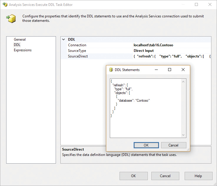
![]() Tip
Tip
It is better to prepare the TMSL command by using the XMLA query pane in SSMS (so you have a minimal editor available) than to try to modify the SourceDirect property directly in the DDL Statements editor (which is the basic text box shown in Figure 11-21).
If you want to parameterize the content of the TMSL command, you must manipulate the SourceDirect property as a string. For example, you can build the TMSL string in a script task by assigning it to a package variable and then using an expression to set the Source property of the task. There is no built-in parameterization feature for the TMSL script in this component.
Using versions of Integration Services earlier than 2016
If you use Integration Services on a version of SQL Server earlier than 2016, you cannot use the Analysis Services Processing task. It supports commands for multidimensional models only and lacks the specific processing commands for a tabular model. Moreover, in previous versions of Integration Services, the TMSL script is not recognized as a valid syntax of an Analysis Services Execute DDL task. In this case, you can specify a TMSL script by wrapping it in an XMLA Statement node, as in the following example:
<Statement xmlns="urn:schemas-microsoft-com:xml-analysis">
{
"refresh": {
"type": "calculate",
"objects": [
{
"database": "Contoso"
}
]
}
}
</Statement>
The TMSL script wrapped in an XMLA Statement node can also run on the latest version of Integration Services (2016).
Using Analysis Management Objects (AMO) and Tabular Object Model (TOM)
You can administer Analysis Services instances programmatically by using the Analysis Management Objects (AMO) API. AMO includes several features that are common to multidimensional and tabular deployments. Specific tabular APIs are usually referenced as Tabular Object Model (TOM), which is an extension of the original AMO client library. Today, however, you could consider TOM a subset of AMO. You might find both terms in the SSAS documentation. You can use AMO and TOM libraries from managed code (such as C# or Visual Basic) or by using PowerShell.
These libraries support the creation of XMLA scripts, or the direct execution of commands on Analysis Services. In this section, you will find a few examples of these capabilities applied to the processing of objects in a tabular model. You will find a more detailed explanation of these libraries in Chapter 13. For a complete example of how to manage rolling partitions, see the “Sample processing scripts” section later in this chapter.
Listing 11-5 shows how you can execute Process Data in C# on the Product and Sales tables, followed by Process Recalc in the same transaction, applying a max parallelism of 5.
Listing 11-5 ModelsChapter 11AmoProcessTablesProgram.cs
using Microsoft.AnalysisServices.Tabular;
namespace AmoProcessTables {
class Program {
static void Main(string[] args) {
Server server = new Server();
server.Connect(@"localhost ab16");
Database db = server.Databases["Contoso"];
Model model = db.Model;
Table tableProduct = model.Tables["Product"];
Table tableSales = model.Tables["Sales"];
tableProduct.RequestRefresh(RefreshType.DataOnly);
tableSales.RequestRefresh(RefreshType.DataOnly);
model.RequestRefresh(RefreshType.Calculate);
model.SaveChanges(new SaveOptions() { MaxParallelism = 5 });
server.Disconnect();
}
}
}
The SaveChanges method called on the Model object is the point where the activities are executed. In practice, all the previous calls to RequestRefresh are simply preparing the list of commands to be sent to Analysis Services. When you call SaveChanges, all the refresh operations are executed in parallel, even if the Process Recalc operation that is applied to the data model always follows the process of other tables and partitions. If you prefer to execute the process commands sequentially, you must call SaveChanges after each RequestRefresh. In other words, SaveChanges executes all the operations requested up to that time.
You can execute the same operations by using PowerShell with script shown in Listing 11-6. You will find more details about these libraries and their use in Chapter 13.
Listing 11-6 Script PowerShellAmoProcessTables.ps1
[System.Reflection.Assembly]::LoadWithPartialName("Microsoft.AnalysisServices.Tabular")
$server = New-Object Microsoft.AnalysisServices.Tabular.Server
$server.Connect("localhost ab16")
$db = $server.Databases["Contoso"]
$model = $db.Model
$tableProduct = $model.Tables["Product"]
$tableSales = $model.Tables["Sales"]
$tableProduct.RequestRefresh("DataOnly")
$tableSales.RequestRefresh("DataOnly")
$model.RequestRefresh("Calculate")
$saveOptions = New-Object Microsoft.AnalysisServices.Tabular.SaveOptions
$saveOptions.MaxParallelism = 5
$model.SaveChanges( $saveOptions )using Microsoft.AnalysisServices.Tabular;
As discussed in the “Using TMSL commands” section, the engine internally converts TMSL into an XMLA script that is specific for Tabular. The AMO library directly generates the XMLA script and sends it to the server, but if you prefer, you can capture this XMLA code instead. You might use this approach to generate valid scripts that you will execute later, even if TMSL would be more compact and readable. (In Chapter 13, you will see a separate helper class in AMO to generate TMSL scripts in JSON.) To capture the XMLA script, enable and disable the CaptureXml property before and after calling the SaveChanges method. Then iterate the CaptureLog property to retrieve the script, as shown in the C# example in Listing 11-7.
Listing 11-7 ModelsChapter 11 AmoProcessTablesScriptProgram.cs
using System;
using Microsoft.AnalysisServices.Tabular;
namespace AmoProcessTables {
class Program {
static void Main(string[] args) {
Server server = new Server();
server.Connect(@"localhost ab16");
Database db = server.Databases["Contoso"];
Model model = db.Model;
Table tableProduct = model.Tables["Product"];
Table tableSales = model.Tables["Sales"];
tableProduct.RequestRefresh(RefreshType.DataOnly);
tableSales.RequestRefresh(RefreshType.DataOnly);
model.RequestRefresh(RefreshType.Calculate);
server.CaptureXml = true;
model.SaveChanges(new SaveOptions() { MaxParallelism = 5 });
server.CaptureXml = false;
// Write the XMLA script on the console
Console.WriteLine("------ XMLA script ------");
foreach (var s in server.CaptureLog) Console.WriteLine(s);
Console.WriteLine("----- End of script -----");
server.Disconnect();
}
}
}
Every call to SaveChanges executes one transaction that includes all the requests made up to that point. If you want to split an operation into multiple transactions, simply call SaveChanges to generate the script or execute the command for every transaction.
Using PowerShell
In addition to using the AMO libraries from PowerShell, you can also use task-specific cmdlets that simplify the code required to perform common operations such as backup, restore, and process. Before starting, you must make sure that specific PowerShell components are installed on the computer where you want to run PowerShell. The simplest way to get these modules is by downloading and installing the latest version of SSMS. The following modules are available:
![]() SQLAS This is for accessing the AMO libraries.
SQLAS This is for accessing the AMO libraries.
![]() SQLASCMDLETS This is for accessing the cmdlets for Analysis Services.
SQLASCMDLETS This is for accessing the cmdlets for Analysis Services.
For a step-by-step guide on installing these components, see https://msdn.microsoft.com/en-us/library/hh213141.aspx.
The following cmdlets are useful for a tabular model:
![]()
Add-RoleMember This adds a member to a database role.
![]()
Backup-ASDatabase This backs up an Analysis Services database.
![]()
Invoke-ASCmd This executes a query or script in the XMLA or TMSL (JSON) format.
![]()
Invoke-ProcessASDatabase This processes a database.
![]()
Invoke-ProcessTable This processes a table.
![]()
Invoke-ProcessPartition This processes a partition.
![]()
Merge-Partition This merges a partition.
![]()
Remove-RoleMember This removes a member from a database role.
![]()
Restore-ASDatabase This restores a database on a server instance.
For a more complete list of available cmdlets and related documentation, see https://msdn.microsoft.com/en-us/library/hh758425.aspx.
Listing 11-8 shows an example of a cmdlet-based PowerShell script that processes the data of two partitions (Sales 2008 and Sales 2009). It then executes a Process Default at the database level, making sure that the database can be queried immediately after that:
Listing 11-8 Script PowerShellCmdlet Process Partitions.ps1
Invoke-ProcessPartition -Server "localhost ab16" -Database "Partitions" -TableName
"Sales"
-PartitionName "Sales 2008" -RefreshType DataOnly
Invoke-ProcessPartition -Server "localhost ab16" -Database "Partitions" -TableName
"Sales"
-PartitionName "Sales 2009" -RefreshType DataOnly
Invoke-ProcessASDatabase -Server "localhost ab16" -DatabaseName "Partitions"
-RefreshType Automatic
Sample processing scripts
This section contains a few examples of processing scripts that you can use as a starting point to create your own versions.
Processing a database
You can process a single database by using a TMSL script. By using the full type in the refresh command, users can query the model just after the process operation. You identify the database by specifying just the database name. The script in Listing 11-9 processes all the tables and partitions of the Static Partitions database.
Listing 11-9 Script TMSLProcess Database.xmla
{
"refresh": {
"type": "full",
"objects": [
{
"database": "Static Partitions",
}
]
}
}
You can obtain the same result using the PowerShell script shown in Listing 11-10. In this case, the script contains the name of the server to which you want to connect (here, localhost ab16).
Listing 11-10 Script PowerShellProcess Database.ps1
[System.Reflection.Assembly]::LoadWithPartialName("Microsoft.AnalysisServices.
Tabular")
$server = New-Object Microsoft.AnalysisServices.Tabular.Server
$server.Connect("localhost ab16")
$db = $server.Databases["Static Partitions"]
$model = $db.Model
$model.RequestRefresh("Full")
$model.SaveChanges()
The PowerShell script retrieves the model object that corresponds to the database to process. (This is identical to the previous TMSL script.) It also executes the RequestRefresh method on it. The call to SaveChanges executes the operation. All the previous lines are required only to retrieve information and to prepare the internal batch that is executed on the server by this method.
Processing tables
You can process one or more tables by using a TMSL script. By using the full type in the refresh command in TMSL, users can query the model just after the process operation. You identify a table by specifying the database and the table name. The script shown in Listing 11-11 processes two tables, Product and Sales, of the Static Partitions database.
Listing 11-11 Script TMSLProcess Tables.xmla
{
"refresh": {
"type": "full",
"objects": [
{
"database": "Static Partitions",
"table": "Product"
},
{
"database": "Static Partitions",
"table": "Sales"
}
]
}
}
You can obtain the same result by using the PowerShell script shown in Listing 11-12. In this case, the script contains the name of the server to which you want to connect (localhost ab16).
Listing 11-12 Script PowerShellProcess Tables.ps1
[System.Reflection.Assembly]::LoadWithPartialName("Microsoft.AnalysisServices.
Tabular")
$server = New-Object Microsoft.AnalysisServices.Tabular.Server
$server.Connect("localhost ab16")
$db = $server.Databases["Static Partitions"]
$model = $db.Model
$tableSales = $model.Tables["Sales"]
$tableProduct = $model.Tables["Product"]
$tableSales.RequestRefresh("Full")
$tableProduct.RequestRefresh("Full")
$model.SaveChanges()
The PowerShell script retrieves the table objects that correspond to the tables to process. (This is identical to the previous TMSL script.) It then executes the RequestRefresh method on each one of them. The call to SaveChanges executes the operation. All the previous lines are required only to retrieve information and to prepare the internal batch that is executed on the server by this method.
Processing partitions
You can process a single partition by using a TMSL script. By using the full type in the refresh command in TMSL, users can query the model just after the process operation. You identify a partition by specifying the database, table, and partition properties. The script in Listing 11-13 processes the Sales 2009 partition in the Sales table of the Static Partitions database.
Listing 11-13 Script TMSLProcess Partition.xmla
{
"refresh": {
"type": "full",
"objects": [
{
"database": "Static Partitions",
"table": "Sales",
"partition": "Sales 2009"
}
]
}
}
You can obtain the same result by using the PowerShell script shown in Listing 11-14. In this case, the script contains the name of the server to which you want to connect (localhost ab16).
Listing 11-14 Script PowerShellProcess Partition.ps1
[System.Reflection.Assembly]::LoadWithPartialName("Microsoft.AnalysisServices.
Tabular")
$server = New-Object Microsoft.AnalysisServices.Tabular.Server
$server.Connect("localhost ab16")
$db = $server.Databases["Static Partitions"]
$model = $db.Model
$tableSales = $model.Tables["Sales"]
$partitionSales2009 = $tableSales.Partitions["Sales 2009"]
$partitionSales2009.RequestRefresh("Full")
$model.SaveChanges()
The PowerShell script retrieves the partition object that corresponds to the partition to process. (This is identical to the previous TMSL script.) It then executes the RequestRefresh method on it. The call to SaveChanges executes the operation. All the previous lines are required only to retrieve information and to prepare the internal batch that is executed on the server by this method.
Rolling partitions
A common requirement is to create monthly partitions in large fact tables, keeping in memory a certain number of years or months. To meet this requirement, the best approach is to create a procedure that automatically generates new partitions, removes old partitions, and processes the last one or two partitions. In this case, you cannot use a simple TMSL script, and you must use PowerShell or some equivalent tool that enables you to analyze existing partitions and to implement a logic based on the current date and the range of months that you want to keep in the tabular model.
The PowerShell script shown in Listing 11-15 implements a rolling partition system for a table with monthly partitions. The script has several functions before the main body of the script. These remove partitions outside of the months that should be online, add missing partitions, and process the last two partitions. The current date implicitly defines the last partition of the interval.
Before the main body of the script, you can customize the behavior of the script by manipulating the following variables:
![]()
$serverName This lists the name of the server, including the instance name.
![]()
$databaseName This lists the name of the database.
![]()
$tableName This lists the name of the table containing the partitions to manage.
![]()
$partitionReferenceName This lists the name of the partition reference.
![]()
$monthsOnline This lists the number of months/partitions to keep in memory.
The data model should be defined with a single partition, called the partition reference. This should include a (1=0) condition in the query’s WHERE predicate. The script then copies the partition reference; clones the partition reference to create one partition for each month; renames the partition with a YYYYMM name (where YYYY is the year and MM the month number); and replaces the (1=0) condition with a SQL predicate that contains only the dates included in the partition (in this example, these are found in the Order Date column). All the partitions are added, removed, and processed in parallel within the same transaction, which corresponds to the execution of the SaveChanges method in the model object.
Listing 11-15 Script PowerShellRolling Partitions.ps1
[System.Reflection.Assembly]::LoadWithPartialName("Microsoft.AnalysisServices.
Tabular")
# Set Verbose to 0 if you do not want to see verbose log
$verbose = 1
function GetPartitionNumber ( [int]$year, [int]$month ) {
$year * 12 - 1 + $month
}
function GetPartitionYear ( $partitionNumber ) {
[int][math]::floor( $partitionNumber / 12)
}
function GetPartitionMonth ( $partitionNumber ) {
[int]( ($partitionNumber ) % 12 + 1)
}
function GetPartitionStart ( $partitionNumber ) {
$year = GetPartitionYear ($partitionNumber )
$month = GetPartitionMonth ($partitionNumber )
(New-Object DateTime( $year, $month, 1 ))
}
function GetPartitionEnd ( $partitionNumber ) {
$year = GetPartitionYear ($partitionNumber )
$month = GetPartitionMonth ($partitionNumber )
(New-Object DateTime( $year, $month, 1 )).AddMonths(1).AddDays(-1)
}
function GetPartitionName ( $partitionNumber ) {
$year = GetPartitionYear ($partitionNumber )
$month = GetPartitionMonth ($partitionNumber )
(New-Object DateTime( $year, $month, 1 )).ToString( "yyyyMM" )
}
function AddPartition( $table, $referencePartition, [int]$partitionNumber ) {
$partitionStart = GetPartitionStart ( $partitionNumber )
$partitionEnd = GetPartitionEnd ( $partitionNumber )
$partitionName = GetPartitionName ( $partitionNumber )
$existingPartition = $table.Partitions.Find($partitionName)
if (!$existingPartition) {
if ($verbose) {
"Add Partition " + $partitionName
}
$placeHolder = "(1=0)"
$newPartitionFilter = '
"([Order Date] BETWEEN '" '
+ $partitionStart.ToString( "yyyyMMdd" ) '
+ "' AND '" + $partitionEnd.ToString( "yyyyMMdd" ) + "')"
$newPartition = $referencePartition.Clone()
$newPartition.Source.Query = $referencePartition.Source.Query.
Replace($placeHolder, $newPartitionFilter )
# $newPartition.Source.Query
$newPartition.Name = $partitionName
$table.Partitions.Add( $newPartition )
}
else {
if ($verbose) {
"Existing Partition=" + $partitionName
}
}
}
function ProcessPartition( $table, [int]$partitionNumber ) {
$partitionName = GetPartitionName ( $partitionNumber )
$existingPartition = $table.Partitions.Find($partitionName)
if (!$existingPartition) {
if ($verbose) {
"Partition not found: " + $partitionName
}
}
else {
if ($verbose) {
"Process table " + $table.Name + " partition " + $partitionName
}
$existingPartition.RequestRefresh("DataOnly")
}
}
function RemovePartition( $table, [int]$partitionNumber ) {
$partitionName = GetPartitionName ( $partitionNumber )
$existingPartition = $table.Partitions.Find($partitionName)
if (!$existingPartition) {
if ($verbose) {
"Partition not found: " + $partitionName
}
}
else {
if ($table.Partitions.Remove($existingPartition)) {
if ($verbose) {
"Removing partition: " + $partitionName
}
}
else {
if ($verbose) {
"Failed remove partition: " + $partitionName
}
}
}
}
# ---------------------------------------------------
# Parameters to process monthly partitions
# ---------------------------------------------------
# Name of the server (including instance name)
$serverName = "localhost ab16"
# Name of the database
$databaseName = "Dynamic Partitions"
#Name of the table containing partitions
$tableName = "Sales"
# Name of partition reference, should contain (1=0) in WHERE condition
$partitionReferenceName = "Sales"
# Number of months/partitions to keep in memory
$monthsOnline = 18
# ---------------------------------------------------
# Script to process monthly partitions
# ---------------------------------------------------
$server = New-Object Microsoft.AnalysisServices.Tabular.Server
$server.Connect( $serverName )
$db = $server.Databases[$databaseName]
$model = $db.Model
$table = $model.Tables[$tableName]
$referencePartition = $table.Partitions[$partitionReferenceName]
# Generate range of partitions to process
$today = Get-Date
# NOTE: The sample database has data between 2007 and 2009.
# By subtracting 8 years, any date in 2017 corresponds
# to dates in 2009. For this reason, we normalize the current
# year so that it corresponds to the last year in the sample database.
# You should remove the AddYears function for your database.
$currentDay = $today.AddYears(2009 - $today.Year)
$lastPartition = $currentDay.Year * 12 - 1 + $currentDay.Month
$firstPartition = $lastPartition - $monthsOnline
# Remove older partitions
ForEach ( $partitionScan in $table.Partitions) {
if ($partitionScan.Name -ne $partitionReferenceName) {
$year = [math]::Floor([int]($partitionScan.Name) / 100)
$month = [int]($partitionScan.Name) % 100
$partitionNumber = GetPartitionNumber $year $month
if ( ($partitionNumber -lt $firstPartition) '
-or ($partitionNumber -gt $lastPartition) ) {
RemovePartition $table $partitionNumber
}
}
}
# Add missing partitions
For ($partitionNumber = $firstPartition; $partitionNumber -le $lastPartition;
$partitionNumber++) {
AddPartition $table $referencePartition $partitionNumber
}
# Process last two partitions
ProcessPartition $table ($lastPartition - 1)
ProcessPartition $table $lastPartition
# Complete refresh at database level (also process new partitions)
$model.RequestRefresh("Automatic")
$model.SaveChanges()
Summary
This chapter discussed how to define and implement partitioning and processing strategies for tabular models. Various APIs and tools can help you in the implementation of your strategy, such as TMSL, AMO, SSIS, and PowerShell. The chapter contained several practical examples for common processing and partitioning operations using TMSL and PowerShell scripts. For more details about the API used by PowerShell scripts, see Chapter 13.