Chapter 3. Loading data inside Tabular
As you learned in Chapter 2, “Getting started with the tabular model,” the key to producing a tabular model is to load data from one or many sources that are integrated in the analysis data model. This enables users to create their reports by browsing the tabular database on the server. This chapter describes the data-loading options available in Tabular mode. You have already used some of the loading features to prepare the examples of the previous chapters. Now you will move a step further and examine all the options for loading data so you can determine which methods are the best for your application.
![]() What’s new in SSAS 2016
What’s new in SSAS 2016
SSAS 2016 offers new impersonation options and a different way to store data copied from the clipboard in the data model.
Understanding data sources
In this section, you learn the basics of data sources, starting with the interfaces between SQL Server Analysis Services (SSAS) and databases. These interfaces provide the abstraction layer that Analysis Services needs to communicate with different sources of data. Analysis Services provides several kinds of data sources, which can be divided into the following categories:
![]() Relational databases Analysis Services can load data hosted in relational databases, such as Microsoft Access, Microsoft SQL Server, Microsoft Azure SQL Database, Oracle, Teradata, Sybase, IBM Informix, IBM DB2, and many others. You can load tables, views, and queries from the server that hosts the data sources in this category.
Relational databases Analysis Services can load data hosted in relational databases, such as Microsoft Access, Microsoft SQL Server, Microsoft Azure SQL Database, Oracle, Teradata, Sybase, IBM Informix, IBM DB2, and many others. You can load tables, views, and queries from the server that hosts the data sources in this category.
![]() Multidimensional sources You can load data into your tabular model from an Analysis Services multidimensional model by using these data sources. Currently, SQL Server Analysis Services is the only multidimensional database for which there is an available data source. The same data source can also load data from queries issued to Power Pivot data contained in a Microsoft Excel workbook that is published on Microsoft SharePoint or from a tabular data model hosted on a server.
Multidimensional sources You can load data into your tabular model from an Analysis Services multidimensional model by using these data sources. Currently, SQL Server Analysis Services is the only multidimensional database for which there is an available data source. The same data source can also load data from queries issued to Power Pivot data contained in a Microsoft Excel workbook that is published on Microsoft SharePoint or from a tabular data model hosted on a server.
![]() Data feeds This category of data sources enables you to load data from dynamic feeds, such as Open Data Protocol (OData) feeds from the Internet, or data feeds tied to reports stored in Reporting Services.
Data feeds This category of data sources enables you to load data from dynamic feeds, such as Open Data Protocol (OData) feeds from the Internet, or data feeds tied to reports stored in Reporting Services.
![]() Text files Data sources in this category can load data that is stored in comma-separated text files, Excel files, fixed-length files, or any other file format that can be interpreted by Analysis Services.
Text files Data sources in this category can load data that is stored in comma-separated text files, Excel files, fixed-length files, or any other file format that can be interpreted by Analysis Services.
![]() Other sources Data can be loaded from the clipboard and stored statically inside the .bim file.
Other sources Data can be loaded from the clipboard and stored statically inside the .bim file.
In a tabular data model, you can freely mix different data sources to load data from various media. It is important to remember that after data is loaded, it must be refreshed by the server on a scheduled basis, depending on your needs, during the database processing.
If you want to see the complete list of all the data sources available in Tabular mode, you can open the Table Import wizard (see Figure 3-1). To do so, open the Model menu and choose Import from Data Source.

The first page of the Table Import wizard lists all the data sources available in Tabular mode. Each data source has specific parameters and dialog boxes. The details for connecting to the specialized data sources can be provided by your local administrator, and are outside the scope of this book. It is interesting to look at the differences between loading from a text file and from a SQL Server query, but it is of little use to investigate the subtle differences between Microsoft SQL Server and Oracle, which are both relational database servers and behave in much the same way.
Understanding impersonation
Some data sources only support what is known as basic authentication, where the user must provide a user name and password in the connection string. For those types of data sources, the impersonation settings are not critical, and you can usually use the service account. Whenever Analysis Services uses Windows authentication to load information from a data source, it must use the credentials of a Windows account so that security can be applied and data access can be granted. Stated more simply, SSAS impersonates a user when opening a data source. The credentials used for impersonation might be different from both the credentials of the user currently logged on—that is, from the user’s credentials—and the ones running the SSAS service.
For this reason, it is very important to decide which user will be impersonated by SSAS when accessing a database. If you fail to provide the correct set of credentials, SSAS cannot correctly access the data, and the server will raise errors during processing. Moreover, the Windows account used to fetch data might be a higher-privileged user, such as a database administrator (DBA), and therefore expose end users to more data from the model than you may have intended. Thus, it is necessary to properly evaluate which credentials should be used.
Moreover, it is important to understand that impersonation is different from SSAS security. Impersonation is related to the credentials the service uses to refresh data tables in the database. In contrast, SSAS security secures the cube after it has been processed, to present different subsets of data to different users. Impersonation comes into play during processing; security is leveraged during querying.
Impersonation is defined on the Impersonation Information page of the Table Import wizard, which is described later (and shown in Figure 3-3). From this page, you can choose the following options:
![]() Specific Windows User Name and Password
Specific Windows User Name and Password
![]() Service Account
Service Account
![]() Current User
Current User
If you use a specific Windows user, you must provide the credentials of a user who will be impersonated by SSAS. If, however, you choose Service Account, SSAS presents itself to the data source by using the same account that runs SSAS (which you can change by using SQL Configuration Manager to update the service parameters in the server). Current User is used only in DirectQuery mode and connects to the data source using the current user logged to Analysis Services, when it is querying the data model. For the purposes of this book, we will focus on the first two options.
Impersonation is applied to each data source. Whether you must load data from SQL Server or from a text file, impersonation is something you must understand and always use to smooth the process of data loading. Each data source can have different impersonation parameters.
It is important, at this point, to digress a bit about the workspace server. As you might recall from Chapter 2, the workspace server hosts the workspace database, which is the temporary database that SQL Server Data Tools (SSDT) uses when developing a tabular solution. If you choose to use Service Account as the user running SSAS, you must pay attention to whether this user is different in the workspace server from the production server, which leads to processing errors. You might find that the workspace server processes the database smoothly, whereas the production server fails.
Understanding server-side and client-side credentials
As you have learned, SSAS impersonates a user when it accesses data. Nevertheless, when you are authoring a solution in SSDT, some operations are executed by the server and others are executed by SSDT on your local machine. Operations executed by the server are called server-side operations, whereas the ones executed by SSDT are called client-side operations. Even if they appear to be executed in the same environment, client and server operations are in fact executed by different software and therefore might use different credentials. The following example should clarify the scenario.
When you import data from SQL Server, you follow the Table Import wizard, by which you can choose the tables to import and preview and filter data. Then, when the selection is concluded, you have loaded data from the database into the tabular model.
The Table Import wizard runs inside SSDT and is executed as a client-side operation. That means it uses the credentials specified for client-side operations—that is, the credentials of the current user. The final data-loading process, however, is executed by the workspace server by using the workspace server impersonation settings, and it is a server-side operation. Thus, in the same logical flow of an operation, you end up mixing client-side and server-side operations, which might lead to different users being impersonated by different layers of the software.
![]() Note
Note
In a scenario that commonly leads to misunderstandings, you specify Service Account for impersonation and try to load some data. If you follow the default installation of SQL Server, the account used to execute SSAS does not have access to the SQL engine, whereas your personal account should normally be able to access the databases. Thus, if you use the Service Account impersonation mode, you can follow the wizard up to when data must be loaded (for example, you can select and preview the tables). At that point, the data loading starts and, because this is a server-side operation, Service Account cannot access the database. This final phase raises an error.
Although the differences between client-side and server-side credentials are difficult to understand, it is important to understand how connections are established. To help you understand the topic, here is a list of the components involved when establishing a connection:
![]() The connection can be initiated by an instance of SSAS or SSDT. You refer to server and client operations, respectively, depending on who initiated the operation.
The connection can be initiated by an instance of SSAS or SSDT. You refer to server and client operations, respectively, depending on who initiated the operation.
![]() The connection is established by using a connection string, defined in the first page of the wizard.
The connection is established by using a connection string, defined in the first page of the wizard.
![]() The connection is started by using the impersonation options, defined on the second page of the wizard.
The connection is started by using the impersonation options, defined on the second page of the wizard.
When the server is trying to connect to the database, it checks whether it should use impersonation. Thus, it looks at what you have specified on the second page and, if requested, impersonates the desired Windows user. The client does not perform this step; it operates under the security context of the current user who is running SSDT. After this first step, the data source connects to the server by using the connection string specified in the first page of the wizard, and impersonation is no longer used at this stage. Therefore, the main difference between client and server operations is that the impersonation options are not relevant to the client operations; they only open a connection through the current user.
This is important for some data sources, such as Access. If the Access file is in a shared folder, this folder must be accessible by both the user running SSDT (to execute the client-side operations) and the user impersonated by SSAS (when processing the table on both the workspace and the deployment servers). If opening the Access file requires a password, both the client and the server use the password stored in the connection string to obtain access to the contents of the file.
Working with big tables
In a tabular project, SSDT shows data from the workspace database in the model window. As you have learned, the workspace database is a physical database that can reside on your workstation or on a server on the network. Wherever this database is, it occupies memory and resources and needs CPU time whenever it is processed.
Processing the production database is a task that can take minutes, if not hours. The workspace database, however, should be kept as small as possible. This is to avoid wasting time whenever you must update it, which happens quite often during development.
To reduce the time it takes, avoid processing the full tables when working with the workspace database. You can use some of the following hints:
![]() You can build a development database that contains a small subset of the production data. That way, you can work on the development database and then, when the project is deployed, change the connection strings to make them point to the production database.
You can build a development database that contains a small subset of the production data. That way, you can work on the development database and then, when the project is deployed, change the connection strings to make them point to the production database.
![]() When loading data from a SQL Server database, you can create views that restrict the number of returned rows, and later change them to retrieve the full set of data when in production.
When loading data from a SQL Server database, you can create views that restrict the number of returned rows, and later change them to retrieve the full set of data when in production.
![]() If you have SQL Server Enterprise Edition, you can rely on partitioning to load a small subset of data in the workspace database and then rely on the creation of new partitions in the production database to hold all the data. You can find further information about this technique at https://blogs.msdn.microsoft.com/cathyk/2011/09/01/importing-a-subset-of-data-using-partitions-step-by-step/.
If you have SQL Server Enterprise Edition, you can rely on partitioning to load a small subset of data in the workspace database and then rely on the creation of new partitions in the production database to hold all the data. You can find further information about this technique at https://blogs.msdn.microsoft.com/cathyk/2011/09/01/importing-a-subset-of-data-using-partitions-step-by-step/.
Your environment and experience might lead you to different mechanisms to handle the size of the workspace database. In general, it is a good practice to think about this aspect of development before you start building the project. This will help you avoid problems later due to the increased size of the workspace model.
Loading from SQL Server
The first data source option is SQL Server. To start loading data from SQL Server, follow these steps:
1. Open the Model menu and choose Import from Data Source to open the Table Import wizard.
2. Select Microsoft SQL Server and click Next.
3. The Connect to a Microsoft SQL Server Database page of the Table Import wizard asks you the parameters by which to connect to SQL Server, as shown in Figure 3-2. Enter the following information and then click Next:
• Friendly Connection Name This is a name that you can assign to the connection to recall it later. We suggest overriding the default name provided by SSDT because a meaningful name will be easier to remember later.
• Server Name This is the name of the SQL Server instance to which you want to connect.
• Log On to the Server This option enables you to choose the method of authentication to use when connecting to SQL Server. You can choose between Use Windows Authentication, which uses the account of the user who is running SSDT to provide the credentials for SQL Server, and Use SQL Server Authentication. In the latter case, you must provide your user name and password in this dialog box. You can also select the Save My Password check box so that you do not have to enter it again during future authentication.
• Database Name In this box, you specify the name of the database to which you want to connect. You can click Test Connection to verify you are properly connected.

4. The Impersonation Information page of the Table Import wizard requires you to specify the impersonation options, as shown in Figure 3-3. Choose from the following options and then click Next:
• Specific Windows User Name and Password SSAS will connect to the data source by impersonating the Windows user specified in these text boxes.
• Service Account SSAS will connect to the data source by using the Windows user running the Analysis Services service.
• Current User This option is used only when you enable the DirectQuery mode in the model.

5. In the Choose How to Import the Data page of the wizard (see Figure 3-4), choose Select from a List of Tables and Views to Choose the Data to Import or Write a Query That Will Specify the Data to Import. Then click Next.

What happens next depends on which option you choose. This is explored in the following sections.
Loading from a list of tables
If you choose to select the tables from a list, the Table Import wizard displays the Select Tables and Views page. This page shows the list of tables and views available in the database, as shown in Figure 3-5. Follow these steps:
1. Click a table in the list to select it for import.
2. Optionally, type a friendly name for the table in the Friendly Name column. This is the name that SSAS uses for the table after it has been imported. (You can change the table name later, if you forget to set it here.)
3. Click the Preview & Filter button to preview the data, to set a filter on which data is imported, and to select which columns to import (see Figure 3-6).


4. To limit the data in a table, apply either of the following two kinds of filters. Both column and data filters are saved in the table definition, so that when you process the table on the server, they are applied again.
• Column filtering You can add or remove table columns by selecting or clearing the check box before each column title at the top of the grid. Some technical columns from the source table are not useful in your data model. Removing them helps save memory space and achieve quicker processing.
• Data filtering You can choose to load only a subset of the rows of the table, specifying a condition that filters out the unwanted rows. In Figure 3-7, you can see the data-filtering dialog box for the Manufacturer column. Data filtering is powerful and easy to use. You can use the list of values that are automatically provided by SSDT. If there are too many values, you can use text filters and provide a set of rules in the forms, such as greater than, less than, equal to, and so on. There are various filter options for several data types, such as date filters, which enable you to select the previous month, last year, and other specific, date-related filters.

![]() Note
Note
Pay attention to the date filters. The query they generate is always relative to the creation date, and not to the execution date. Thus, if you select Last Month, December 31, you will always load the month of December, even if you run the query on March. To create queries relative to the current date, rely on views or author-specific SQL code.
5. When you finish selecting and filtering the tables, click Finish for SSDT to begin processing the tables in the workspace model, which in turn fires the data-loading process. During the table processing, the system detects whether any relationships are defined in the database, among the tables currently being loaded, and, if so, the relationships are loaded inside the data model. The relationship detection occurs only when you load more than one table.
6. The Work Item list, in the Importing page of the Table Import wizard, is shown in Figure 3-8. On the bottom row, you can see an additional step, called Data Preparation, which indicates that relationship detection has occurred. If you want to see more details about the found relationships, you can click the Details hyperlink to open a small window that summarizes the relationships created. Otherwise, click Close.

Figure 3-8 The Data Preparation step of the Table Import wizard, showing that relationships have been loaded.
Loading from a SQL query
If you chose the Write a Query That Will Specify the Data to Import option in the Choose How to Import the Data page of the Table Import wizard (refer to Figure 3-4), you have two choices:
![]() Write the query in a simple text box You normally would paste it from a SQL Server Management Studio (SSMS) window, in which you have already developed it.
Write the query in a simple text box You normally would paste it from a SQL Server Management Studio (SSMS) window, in which you have already developed it.
![]() Use the Table Import wizard’s query editor to build the query This is helpful if you are not familiar with SQL Server.
Use the Table Import wizard’s query editor to build the query This is helpful if you are not familiar with SQL Server.
To use the query editor, click the Design button in the Table Import wizard. The Table Import wizard’s query editor is shown in Figure 3-9.

Figure 3-9 The Table Import wizard’s query editor, which enables you to design a SQL query visually as the data source.
Loading from views
Because you have more than one option by which to load data (a table or SQL query), it is useful to have guidance on which method is the best one. The answer is often neither of these methods.
Linking the data model directly to a table creates an unnecessary dependency between the tabular data model and the database structure. In the future, it will be harder to make any change to the physical structure of the database. However, writing a SQL query hides information about the data source within the model. Neither of these options seems to be the right one.
It turns out, as in the case of multidimensional solutions, that the best choice is to load data from views instead of from tables. You gain many advantages by using views. Going into the details of these advantages is outside the scope of this book, but we will provide a high-level overview (you can find a broader discussion about best practices in data import that is valid also for Analysis Services at https://www.sqlbi.com/articles/data-import-best-practices-in-power-bi/). The advantages can be summarized in the following way:
![]() Decoupling the physical database structure from the tabular data model
Decoupling the physical database structure from the tabular data model
![]() Declarative description in the database of the tables involved in the creation of a tabular entity
Declarative description in the database of the tables involved in the creation of a tabular entity
![]() The ability to add hints, such as NOLOCK, to improve processing performance
The ability to add hints, such as NOLOCK, to improve processing performance
Thus, we strongly suggest you spend some time defining views in your database, each of which will describe one entity in the tabular data model. Then you can load data directly from those views. By using this technique, you will get the best of both worlds: the full power of SQL to define the data to be loaded without hiding the SQL code in the model definition.
Importing data from views is also a best practice in Power Pivot and Power BI. To improve usability, in these views you should include spaces between words in a name and exclude prefixes and suffixes. That way, you will not spend time renaming names in Visual Studio. An additional advantage in a tabular model is that the view simplifies troubleshooting because if the view has exactly the same names of tables and columns used in the data model, then any DBA can run the view in SQL Server to verify whether the lack of some data is caused by the Analysis Services model or by missing rows in the data source.
Opening existing connections
In the preceding section, you saw all the steps and options of data loading, by creating a connection from the beginning. After you create a connection with a data source, it is saved in the data model so that you can open it without providing the connection information again. This option is available from the Model menu under Existing Connections.
Choosing this option opens the Existing Connections dialog box shown in Figure 3-10, in which you can select the connections saved in the model. From this window, you can choose a connection and then decide to use the connection to load data from other tables, to edit the connection parameters, to delete the connection, or to process all the tables linked to that connection.

Figure 3-10 The Existing Connections dialog box, which lists all the connections saved in the project.
It is very important to become accustomed to reopening existing connections whenever you must import more tables from the same database. That way, if you create a new connection each time you intend to load data, you create many connections in the same model. If you have many connections, and you need to modify some of the connection parameters, you will have extra work to update all the connections.
Loading from Access
Now that you have seen all the ways that data can be loaded from relational databases, you can examine other data sources, the first of which is the Access data source.
When you open the Table Import wizard by using the Access data source, the connection parameters are different because the Access databases are stored in files on disk instead of being hosted in server databases. In Figure 3-11, you can see the Table Import wizard requesting that you identify an Access file.

There is no practical difference between Access and any other relational database in loading tables, but be aware that the server uses the 64-bit Access Database Engine (ACE) driver, whereas in SSDT, you are using the 32-bit version. It is worth noting that the SQL Server designer of Access is limited because it does not offer a visual designer for the SQL query. When you query Access, you must write the query in a plain text editor.
Because the Table Import wizard for Access does not have a query designer, if you must load data from Access and need help with SQL, it might be better to write the query by using the query designer from inside Access. Then, after the query has been built in Access, you can load the data from that query. By doing so, you add an abstraction layer between the Access database and the tabular data model, which is always a best practice to follow.
When using an Access data source, pay attention to the following points:
![]() The file path should point to a network location that the server can access when it processes the data model.
The file path should point to a network location that the server can access when it processes the data model.
![]() When processing the table, the user that is impersonated by the SSAS engine should have enough privileges to be able to access that folder.
When processing the table, the user that is impersonated by the SSAS engine should have enough privileges to be able to access that folder.
![]() The workspace database uses the ACE driver installed on that server, so be aware of the bit structure of SSAS versus the bit structure of Office.
The workspace database uses the ACE driver installed on that server, so be aware of the bit structure of SSAS versus the bit structure of Office.
If the file is password protected, you should enter the password on the first page of the wizard and save it in the connection string so that the SSAS engine can complete the processing without errors.
Loading from Analysis Services
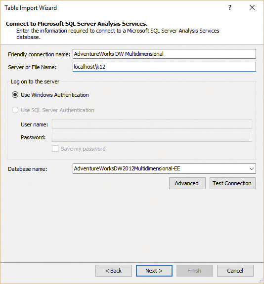
In the preceding sections, you learned how to load data from relational databases. Different relational data sources might have some slight differences among them, but the overall logic of importing from a relational database remains the same. This section explains the SQL Server Analysis Services data source, which has some unique features.
In the Table Import wizard for SSAS (see Figure 3-12), you must provide the server name and the database to which you want to connect.
Click Next on the first page to open the Multidimensional Expressions (MDX) query editor. The MDX editor is similar to the SQL editor. It contains a simple text box, but the language you must use to query the database is MDX instead of SQL. You can write MDX code in the text box or paste it from an SSMS window in which you have already developed and tested it. As with the SQL editor, you do not need to know the MDX language to build a simple query. SSDT contains an advanced MDX query designer, which you can open by clicking the Design button.
![]() Note
Note
As you might have already noticed, you cannot import tables from an Analysis Services database. The only way to load data from an Analysis Services database is to write a query. The reason is very simple: Online analytical processing (OLAP) cubes do not contain tables, so there is no option for table selection. OLAP cubes are composed of measure groups and dimensions, and the only way to retrieve data from these is to create an MDX query that creates a dataset to import.
Using the MDX editor
Using the MDX editor (see Figure 3-13) is as simple as dragging measures and dimensions into the result panel, and it is very similar to querying a multidimensional cube by using Excel. After you have designed the query, click OK; the user interface returns to the query editor, showing the complex MDX code that executes the query against the server.

Because this book is not about MDX, it does not include a description of the MDX syntax or MDX capabilities. The interested reader can find several good books about the topic from which to start learning MDX, such as Microsoft SQL Server 2008 MDX Step by Step by Brian C. Smith and C. Ryan Clay (Microsoft Press), MDX Solutions with Microsoft SQL Server Analysis Services by George Spofford (Wiley), and MDX with SSAS 2012 Cookbook by Sherry Li (Packt Publishing). A good reason to learn MDX is to use the MDX editor to define new calculated members, which help you load data from the SSAS cube. A calculated member is similar to a SQL calculated column, but it uses MDX and is used in an MDX query.
If you have access to an edition of Analysis Services that supports DAX queries over a multidimensional model, you can also write a DAX query, as explained in the next section, “Loading from a tabular database.”
![]() More Info
More Info
Analysis Services 2016 supports the ability to perform a DAX query over a multidimensional model in all available editions (Standard and Enterprise). However, Analysis Services 2012 and 2014 require the Business Intelligence edition or the Enterprise edition. Analysis Services 2012 also requires Microsoft SQL Server 2012 Service Pack 1 and Cumulative Update 2 or a subsequent update.
Loading from a tabular database
As you have learned, you can use the SSAS data source to load data from a multidimensional database. An interesting and, perhaps, not-so-obvious feature is that you can use the same data source to load data from a tabular data model. The tabular model can be either a tabular database in SSAS or a Power Pivot workbook hosted in Power Pivot for SharePoint.
To load data from Tabular mode, you connect to a tabular database in the same way you connect to a multidimensional one. The MDX editor shows the tabular database as if it were multidimensional, exposing the data in measure groups and dimensions, even if no such concept exists in a tabular model. In Figure 3-14, you can see the MDX editor open over the tabular version of the Adventure Works SSAS database.

At this point, you might be wondering whether you can query a tabular database using DAX. After all, DAX is the native language of Tabular mode, and it seems odd to be able to load data from Tabular mode by using MDX only. It turns out that this feature, although well hidden, is indeed available. The MDX editor is not capable of authoring or understanding DAX queries. Nevertheless, because the SSAS server in Tabular mode understands both languages, you can write a DAX query directly in the Table Import wizard in the place of an MDX statement, as shown in Figure 3-15.

The DAX query shown in Figure 3-15 is a very simple one. It loads the sales aggregated by year and model name. When you click the Validate button, the message, “The MDX statement is valid” appears, even if the query is in DAX. In reality, Analysis Services accepts both languages, even if the dialog box does not acknowledge that.
Authoring the DAX query inside the small text box provided by the Table Import wizard is not very convenient. Nevertheless, you can prepare the DAX query inside DAX Studio and then paste it inside the text box.
When using DAX to query the tabular data model, the column names assigned by the data source contain the table name as a prefix (if they come from a table). They represent the full name if they are introduced by the query. For example, the query in Figure 3-15 produces the results shown in Figure 3-16.

The DateCalendar Year and ProductModel Name columns must be adjusted later, removing the table name and renaming them to Calendar Year and Model Name, but the Total Sales column is already correct. A possible workaround is using the SELECTCOLUMNS function to rename the column names in DAX, but such a function is available only when querying an Analysis Services 2016 server. It is not available in previous versions of Analysis Services.
Loading from an Excel file
Data such as budgets or predicted sales is often hosted inside Excel files. In such cases, you can load the data directly from the Excel workbook into the tabular data model.
It might be worthwhile to write an Integration Services package to load that Excel workbook into a database and keep historical copies of it. Tabular models are intended for corporate business intelligence (BI), so you likely will not need to load data from Excel as often as self-service users do. There are a few issues to look out for when loading data from Excel. If you are loading from a range in which the first few rows are numeric, but further rows are strings, the driver might interpret those rows as numeric and return the string values as null. However, the rest of this section explains possible workarounds if you insist on loading from Excel.
Suppose that you have an Excel workbook that contains predicted sales in an Excel table named PredictedSales, as shown in Figure 3-17. To load this workbook into the tabular data model, follow these steps:

1. Open the Table Import wizard.
2. Select the Excel data source and click Next. This opens the page shown in Figure 3-18.

3. In the Excel File Path box, type the file path of the file containing the data.
4. If your table contains column names in the first row (as is the case in this example), select the Use First Row as Column Headers check box to ensure that SSDT automatically detects the column names of the table. Then click Next.
5. In the Impersonation page, leave the settings as is, and click Next.
6. In the Select Tables and Views page (see Figure 3-19), define the worksheets and/or ranges from the workbook to load inside the data model.
![]() Important
Important
Only worksheets and named ranges are imported from an external Excel workbook. If multiple Excel tables are defined on a single sheet, they are not considered. For this reason, it is better to have only one table for each worksheet and no other data in the same worksheet. SSDT cannot detect Excel tables in a workbook. The wizard automatically removes blank space around your data.
7. The wizard loads data into the workspace data model. You can click the Preview & Filter button to look at the data before the data loads and then apply filtering, as you learned to do with relational tables. When you are finished, click Finish.

Similar to Access files, you must specify a file path that will be available to the server when processing the table, so you should not use local resources of the development workstation (such as the C: drive), and you must check that the account impersonated by SSAS has enough privileges to reach the network resource in which the Excel file is located.
Loading from a text file
A common data format from which to load is text files. Data in text files often comes in the form of comma separated values (CSV), a common format by which each column is separated from the previous one by a comma, and a newline character is used as the row separator.
If you have a CSV file that contains some data, you can import it into the data model by using the text file data source. If your CSV file contains the special offers planned for the year 2005, it might look like the following data sample:
Special Offer,Start,End,Category,Discount
Christmas Gifts,12/1/2005,12/31/2005,Accessory,25%
Christmas Gifts,12/1/2005,12/31/2005,Bikes,12%
Christmas Gifts,12/1/2005,12/31/2005,Clothing,24%
Summer Specials,8/1/2005,8/15/2005,Clothing,10%
Summer Specials,8/1/2005,8/15/2005,Accessory,10%
Usually, CSV files contain the column header in the first row of the file, so that the file includes the data and the column names. This is the same standard you normally use with Excel tables.
To load this file, follow these steps:
1. Start the Table Import wizard.
2. Choose the Text File data source and click Next. The Connect to Flat File page of the Table Import wizard (see Figure 3-20) contains the basic parameters used to load from text files.

3. Choose the column separator, which by default is a comma, from the Column Separator list. This list includes Comma, Colon, Semicolon, Tab, and several other separators. The correct choice depends on the column separator that is used in the text file.
Handling more complex CSV files
You might encounter a CSV file that contains fancy separators and find that the Table Import wizard cannot load it correctly because you cannot choose the necessary characters for the separators. It might be helpful, in such a case, to use the schema.ini file, in which you can define advanced properties of the comma separated file. Read https://msdn.microsoft.com/en-us/library/ms709353.aspx to learn this advanced technique for loading complex data files. At the same link, you will find information about how to load text files that do not follow the CSV schema, but use a fixed width instead.
1. If your CSV file contains column names in the first row, select the Use First Row as Column Headers check box to ensure that SSDT automatically detects the column names of the table. (By default, this check box is cleared, even if most CSV files follow this convention and contain the column header.) Then click Next.
2. As soon as you fill the parameters, the grid shows a preview of the data. You can use the grid to select or clear any column and to set row filters, as you can do with any other data source you have seen. When you finish the setup, click Finish to start the loading process.
![]() Note
Note
After the loading is finished, check the data to see whether the column types have been detected correctly. CSV files do not contain, for instance, the data type of each column, so SSDT tries to determine the types by evaluating the file content. Because SSDT is making a guess, it might fail to detect the correct data type. In the example, SSDT detected the correct type of all the columns except the Discount column. This is because the flat file contains the percentage symbol after the number, causing SSDT to treat it as a character string and not as a number. If you must change the column type, you can do that later by using SSDT or, in a case like this example, by using a calculated column to get rid of the percentage sign.
Loading from the clipboard
This section explains the clipboard data-loading feature. This method of loading data inside a tabular database has some unique behaviors—most notably, the fact that it does not rely on a data source.
To load data from the clipboard, follow these steps:
1. Open a sample workbook (such as the workbook shown in Figure 3-17).
2. Copy the Excel table content into the clipboard.
3. In SSDT, from inside a tabular model, open the Edit menu and choose Paste. SSDT analyzes the contents of the clipboard.
4. If the contents contain valid tabular data, SSDT opens the Paste Preview dialog box (see Figure 3-21). It displays the clipboard as it will be loaded inside a tabular table. You can give the table a meaningful name and preview the data before you import it into the model. Click OK to end the loading process and to place the table in the data model.

You can initiate the same process by copying a selection from a Word document or from any other software that can copy data in the tabular format to the clipboard.
How will the server be able to process such a table if no data source is available? Even if data can be pushed inside the workspace data model from SSDT, when the project is deployed to the server, Analysis Services will reprocess all the tables, reloading the data inside the model. It is clear that the clipboard content will not be available to SSAS. Thus, it is interesting to understand how the full mechanism works in the background.
If the tabular project contains data loaded from the clipboard, this data is saved in the DAX expression that is assigned to a calculated table. The expression uses the DATATABLE function, which creates a table with the specified columns, data types, and static data for the rows that populate the table. As shown in Figure 3-22, the Predictions table is imported in the data model, with the corresponding DAX expression that defined the structure and the content of the table itself.

![]() Note
Note
In compatibility levels lower than 1200, a different technique is used to store static data that is pasted in the data model. It creates a special connection that reads the data saved in a particular section of the .bim file, in XML format. In fact, calculated tables are a new feature in the 1200 compatibility level. In SSDT, linked tables are treated much the same way as the clipboard is treated, but when you create a tabular model in SSDT by starting from a Power Pivot workbook, the model is created in the compatibility level 110x, so the former technique is applied. This means linked tables cannot be refreshed when the Excel workbook is promoted to a fully featured tabular solution. If you upgrade the data model to 1200, these tables are converted into calculated tables, exposing the content in the DAX expression that is assigned to the table.
Although this feature looks like a convenient way of pushing data inside a tabular data model, there is no way, apart from manually editing the DAX expression of the calculated table, to update this data later. In a future update of SSDT (this book currently covers the November 2016 version), a feature called Paste Replace will allow you to paste the content of the clipboard into a table created with a Paste command, overwriting the existing data and replacing the DATATABLE function call.
Moreover, there is absolutely no way to understand the source of this set of data later on. Using this feature is not a good practice in a tabular solution that must be deployed on a production server because all the information about this data source is very well hidden inside the project. A much better solution is to perform the conversion from the clipboard to a table (when outside of SSDT), create a table inside SQL Server (or Access if you want users to be able to update it easily), and then load the data inside tabular from that table.
We strongly discourage any serious BI professional from using this feature, apart from prototyping. (For prototyping, it might be convenient to use this method to load the data quickly inside the model to test the data.) Nevertheless, tabular prototyping is usually carried out by using Power Pivot for Excel. There you might copy the content of the clipboard inside an Excel table and then link it inside the model. Never confuse prototypes with production projects. In production, you must avoid any hidden information to save time later when you will probably need to update some information.
There is only one case when using this feature is valuable for a production system: if you need a very small table with a finite number of rows, with a static content set that provides parameters for the calculations that are used in specific DAX measures of the data model. You should consider that the content of the table is part of the structure of the data model, in this case. So to change it, you must deploy a new version of the entire data model.
Loading from a Reporting Services report
When you work for a company, you are likely to have many reports available to you. You might want to import part or all of the data of an existing report into your model.
You might be tempted to import the data by copying it manually or by using copy-and-paste techniques. However, these methods mean that you always load the final output of the report and not the original data that has been used to make the calculations. Moreover, if you use the copy-and-paste technique, you often have to delete the formatting values from the real data, such as separators, labels, and so on. In this way, it is difficult—if not impossible—to build a model that can automatically refresh the data extracted from another report; most of the time, you end up repeating the import process of copying data from your sources.
If you are using reports published by SQL Server Reporting Services 2008 R2 and later, SSAS can connect directly to the data the report uses. In this way, you have access to a more detailed data model, which can also be refreshed. Furthermore, you are not worried by the presence of separators or other decorative items that exist in the presentation of the report. You get only the data. In fact, you can use a report as a special type of data feed, which is a more general type of data source described in the next section. You can import data from Reporting Services in two ways: using a dedicated user interface in SSDT or through the data feed output in the report itself.
Loading reports by using the report data source
Look at the report shown in Figure 3-23. The URL in the Web browser, at the top of the image, points to a sample Reporting Services report. (The URL can be different, depending on the installation of Reporting Services sample reports, which you can download from http://msftrsprodsamples.codeplex.com/.)

This report shows the sales divided by region and by individual stores using a chart and a table. If you click the Number of Stores column’s number of a state, the report scrolls down to the list of shops in the corresponding state. So you see another table, not visible in Figure 3-23, which appears when you scroll down the report.
You can import data from a report inside SSDT by using the report data source. Follow these steps:
1. Start the Table Import wizard.
2. On the Connect to a Data Source page, select Report and click Next. This opens the Connect to a Microsoft SQL Server Reporting Services Report page of the Table Import wizard (see Figure 3-24).

3. Click the Browse button next to the Report Path box and select the report to use, as shown in Figure 3-25.

4. Click Open. The selected report appears in the Table Import wizard, as shown in Figure 3-26.

5. Optionally, you can change the friendly connection name for this connection. Then click Next.
6. Set up the impersonation options to instruct which user SSAS has to use to access the report when refreshing data and click Next.
7. The Select Tables and Views page opens. Choose which data table to import from the report, as shown in Figure 3-27. The report shown here contains four data tables. The first two contain information about the graphical visualization of the map, on the left side of the report in Figure 3-26. The other two are interesting: Tablix1 is the source of the table on the right side, which contains the sales divided by state, and tblMatrix_StoresbyState contains the sales of each store for each state.

8. The first time you import data from a report, you might not know the content of each of the available data tables. In this case, you can click the Preview & Filter button to preview the table. (Figure 3-28 shows the preview.) Or, you can click Finish to import everything, and then remove all the tables and columns that do not contain useful data.

![]() Note
Note
You can see in Figure 3-28 that the last two columns do not have meaningful names. These names depend on the discipline of the report author. Because they usually are internal names that are not visible in a report, it is common to have such non-descriptive names. In such cases, you should rename these columns before you use these numbers in your data model.
Now that you have imported the report data into the data model, the report will be queried again each time you reprocess it, and the updated data will be imported to the selected tables, overriding previously imported data.
Loading reports by using data feeds
You have seen how to load data from a report by using the Table Import wizard for the report data source. There is another way to load data from a report, however: by using data feeds. Follow these steps:
1. Open the report that contains the data you want to load in the Reporting Services web interface.
2. Click the Save button and choose Data Feed from the export menu that appears, as shown in Figure 3-29. Your browser will save the report as a file with the .atomsvc extension.

Figure 3-29 The Reporting Services web interface, showing the Data Feed item in the export drop-down menu (Save).
The .atomsvc file contains technical information about the source data feeds. This file is a data service document in an XML format that specifies a connection to one or more data feeds.
3. Start the Table Import wizard.
4. On the Connect to a Data Source page, choose Other Feeds and then click Next.
5. In the Connect to a Data Feed page of the Table Import wizard, click the Browse button next to the Data Feed URL box. Then select the .atomsvc file you saved in step 2. Figure 3-30 shows the result.

Figure 3-30 Providing the path to the .atomsvc file in the Table Import wizard’s Connect to a Data Feed page.
6. Click Next. Then repeat steps 5–8 in the preceding section.
Loading report data from a data feed works exactly the same way as loading it directly from the report. You might prefer the data feed when you are already in a report and you do not want to enter the report parameters again, but it is up to you to choose the one that fits your needs best.
![]() Note
Note
After the .atomsvc file has been used to grab the metadata information, you can safely remove it from your computer because SSDT does not use it anymore.
Loading from a data feed
In the previous section, you saw how to load a data feed exported by Reporting Services in Tabular mode. However, this technique is not exclusive to Reporting Services. It can be used to get data from many other services. This includes Internet sources that support the Open Data Protocol (OData; see http://odata.org for more information) and data exported as a data feed by SharePoint 2010 and later (described in the next section).
![]() Note
Note
Analysis Services supports OData until version 3. It does not yet support version 4.
To load from one of these other data feeds, follow these steps:
1. Start the Table Import wizard.
2. On the Connect to a Data Source page, click Other Feeds and then click Next.
3. The Connect to a Data Feed page of the Table Import wizard (shown in Figure 3-31) requires you to enter the data feed URL. You saw this dialog box in Figure 3-30, when you were getting data from a report. This time, however, the Data Feed URL box does not have a fixed value provided by the report itself. Instead, you enter the URL of whatever source contains the feed you want to load. In this example, you can use the following URL to test this data source:
http://services.odata.org/V3/OData/OData.svc/

4. Optionally, you can change the friendly connection name for this connection. Then click Next.
5. Set up the impersonation options to indicate which user SSAS must use to access the data feed when refreshing data and then click Next.
6. Select the tables to import (see Figure 3-32), and then follow a standard table-loading procedure.

7. Click Finish. The selected tables are imported into the data model. This operation can take a long time if you have a high volume of data to import and if the remote service that is providing the data has a slow bandwidth.
Loading from SharePoint
Microsoft SharePoint might contain several instances of data you would like to import into your data model. There is no specific data source dedicated to importing data from SharePoint. Depending on the type of data or the document you want to use, you must choose one of the methods already shown.
A list of the most common data sources you can import from SharePoint includes the following:
![]() Report A report generated by Reporting Services can be stored and displayed in SharePoint. In this case, you follow the same procedure described in the “Loading from a Reporting Services report” section earlier in this chapter, by providing the report pathname or by using OData.
Report A report generated by Reporting Services can be stored and displayed in SharePoint. In this case, you follow the same procedure described in the “Loading from a Reporting Services report” section earlier in this chapter, by providing the report pathname or by using OData.
![]() Excel workbook You can import data from an Excel workbook that is saved in SharePoint, the same way you would if it were saved on disk. Refer to the “Loading from an Excel file” section earlier in this chapter, and use the path to the library that contains the Excel file that you want.
Excel workbook You can import data from an Excel workbook that is saved in SharePoint, the same way you would if it were saved on disk. Refer to the “Loading from an Excel file” section earlier in this chapter, and use the path to the library that contains the Excel file that you want.
![]() Power Pivot model embedded in an Excel workbook If an Excel workbook contains a Power Pivot model and is published in a Power Pivot folder, you can extract data from the model by querying it. To do that, you can follow the same steps described in the “Loading from Analysis Services” section earlier in this chapter, with the only difference being that you use the complete path to the published Excel file instead of the name of an Analysis Services server. (You do not have a Browse help tool; you probably need to copy and paste the complete URL from a browser.)
Power Pivot model embedded in an Excel workbook If an Excel workbook contains a Power Pivot model and is published in a Power Pivot folder, you can extract data from the model by querying it. To do that, you can follow the same steps described in the “Loading from Analysis Services” section earlier in this chapter, with the only difference being that you use the complete path to the published Excel file instead of the name of an Analysis Services server. (You do not have a Browse help tool; you probably need to copy and paste the complete URL from a browser.)
![]() SharePoint list Any data included in a SharePoint list can be exported as a data feed. So you can use the same instructions described in the “Loading from a Reporting Services report” and “Loading from a data feed” sections earlier in this chapter. When you click the Export as Data Feed button in SharePoint, an .atomsvc file is downloaded, and you see the same user interface previously shown for reports.
SharePoint list Any data included in a SharePoint list can be exported as a data feed. So you can use the same instructions described in the “Loading from a Reporting Services report” and “Loading from a data feed” sections earlier in this chapter. When you click the Export as Data Feed button in SharePoint, an .atomsvc file is downloaded, and you see the same user interface previously shown for reports.
Choosing the right data-loading method
SSDT makes many data sources available, each with specific capabilities and scenarios of usage. Nevertheless, as seasoned BI professionals, we (the authors) think it is important to warn our readers about some issues they might encounter during the development of a tabular solution.
The problems with the clipboard method of loading data were discussed earlier. The fact that it is not reproducible should discourage you from adopting it in a production environment. The only exception is loading very small tables with fixed lists of parameters to be used in particular measures.
Other data sources should be used only with great care. Whenever you develop a BI solution that must be processed by SSAS, you must use data sources that are the following:
![]() Well typed Each column should have a data type clearly indicated by the source system. Relational databases normally provide this information. Other sources, such as CSV files, Excel workbooks, and the clipboard, do not. SSDT infers this information by analyzing the first few rows of data and assumes the rest of the data matches that type. However, it might be the case that later rows contain different data types, which will cause the loading process to fail.
Well typed Each column should have a data type clearly indicated by the source system. Relational databases normally provide this information. Other sources, such as CSV files, Excel workbooks, and the clipboard, do not. SSDT infers this information by analyzing the first few rows of data and assumes the rest of the data matches that type. However, it might be the case that later rows contain different data types, which will cause the loading process to fail.
![]() Consistent The data types and columns should not change over time. For example, if you use an Excel workbook as the data source, and you let users freely update the workbook, then you might encounter a situation in which the workbook contains the wrong data or the user has changed the column order. SSAS will not handle these changes automatically, and the data will not be loaded successfully.
Consistent The data types and columns should not change over time. For example, if you use an Excel workbook as the data source, and you let users freely update the workbook, then you might encounter a situation in which the workbook contains the wrong data or the user has changed the column order. SSAS will not handle these changes automatically, and the data will not be loaded successfully.
![]() Time predictable Some data sources, such as certain OData feeds, might take a very long time to execute. Just how long this takes will vary depending on the network bandwidth available and any problems with the Internet connection. This might make the processing time quite unpredictable, or it might create problems due to timeouts.
Time predictable Some data sources, such as certain OData feeds, might take a very long time to execute. Just how long this takes will vary depending on the network bandwidth available and any problems with the Internet connection. This might make the processing time quite unpredictable, or it might create problems due to timeouts.
![]() Verified If the user can freely update data, as is the case in Excel workbooks, the wrong data might be added to your tabular data model, which would produce unpredictable results. Data entering Analysis Services should always be double-checked by some kind of software that ensures its correctness.
Verified If the user can freely update data, as is the case in Excel workbooks, the wrong data might be added to your tabular data model, which would produce unpredictable results. Data entering Analysis Services should always be double-checked by some kind of software that ensures its correctness.
For these reasons, we discourage our readers from using the following data sources:
![]() Excel The data is often not verified, not consistent, and not well typed.
Excel The data is often not verified, not consistent, and not well typed.
![]() Text file The data is often not well typed.
Text file The data is often not well typed.
![]() OData The data is often not time predictable when the data comes from the web.
OData The data is often not time predictable when the data comes from the web.
For all these kinds of data sources, a much better solution is to create some kind of extract, transform, load (ETL) process that loads the data from these sources, cleans the data, and verifies that the data is valid and available. Then it puts all the information inside tables in a relational database (such as SQL Server), from which you can feed the tabular data model.
Summary
In this chapter, you were introduced to all the various data-loading capabilities of Tabular mode. You can load data from many data sources, which enables you to integrate data from the different sources into a single, coherent view of the information you must analyze.
The main topics you must remember are the following:
![]() Impersonation SSAS can impersonate a user when opening a data source, whereas SSDT always uses the credentials of the current user. This can lead to server-side and client-side operations that can use different accounts for impersonation.
Impersonation SSAS can impersonate a user when opening a data source, whereas SSDT always uses the credentials of the current user. This can lead to server-side and client-side operations that can use different accounts for impersonation.
![]() Working with big tables When you are working with big tables, the data needs to be loaded in the workspace database. Therefore, you must limit the number of rows that SSDT reads and processes in the workspace database so that you can work safely with your solution.
Working with big tables When you are working with big tables, the data needs to be loaded in the workspace database. Therefore, you must limit the number of rows that SSDT reads and processes in the workspace database so that you can work safely with your solution.
![]() Data sources There are many data sources to connect to different databases. Choosing the right one depends on your source of data. That said, if you must use one of the discouraged sources, remember that if you store data in a relational database before moving it into Tabular mode, you permit data quality control, data cleansing, and more predictable performances.
Data sources There are many data sources to connect to different databases. Choosing the right one depends on your source of data. That said, if you must use one of the discouraged sources, remember that if you store data in a relational database before moving it into Tabular mode, you permit data quality control, data cleansing, and more predictable performances.