Chapter 2. Getting started with the tabular model

Now that you have been introduced to the Analysis Services tabular model, this chapter shows you how to get started developing tabular models yourself. You will discover how to install Analysis Services, how to work with projects in SQL Server Data Tools, what the basic building blocks of a tabular model are, and how to build, deploy, and query a very simple tabular model.

A development workstation

A development server

A workspace database, which might be hosted on a separate workspace server

You may install each of these components on separate machines or on a single machine. Each component has a distinct role to play, and it is important for you to understand these roles.

To create and modify a tabular model, SSDT needs a workspace database. This is a temporary data-base that can be created on the same development workstation using Integrated Workspace Mode or on a specific instance of Analysis Services. (For more on this, see the section “Workspace database server installation” later in this chapter.)

After you finish designing your tabular model in SSDT, you must build and deploy your project. Building a project is like compiling code. The build process translates all the information stored in the files in your project into a data definition language called Tabular Model Scripting Language (TMSL). Deployment involves executing this TMSL on the Analysis Services tabular instance running on your development server. The result will either create a new database or alter an existing database.

A development server should be in the same domain as your development workstation. After you deploy your project to your development server, you and anyone else to whom you give permission will be able to see your tabular model and query it. This will be especially important for any other members of your team who are building reports or other parts of your BI solution.

Your development workstation and your development server can be two machines, or you can use the same machine for both roles. It is best, however, to use a separate, dedicated machine as your development server for the following reasons:

A dedicated server will likely have a much better hardware specification than a workstation. In particular, as you will soon see, the amount of available memory can be very important when developing with tabular. Memory requirements also mean that using a 64-bit operating system is important. Nowadays, you can almost take this for granted on new servers and workstations, but you might still find legacy computers with 32-bit versions of Windows.

A dedicated server will make it easy for you to grant access to your tabular models to other developers, testers, or users while you work. This enables them to run their own queries and build reports without disturbing you. Some queries can be resource-intensive, and you will not want your workstation grinding to a halt unexpectedly when someone else runs a huge query. And, of course, no one would be able to run queries on your workstation if you have turned it off and gone home for the day.

A dedicated server will enable you to reprocess your models while you perform other work. As noted, reprocessing a large model is very resource-intensive and could last for several hours. If you try to do this on your own workstation, it is likely to stop you from doing anything else.

A dedicated development server will (probably) be backed up regularly. This reduces the likelihood that hardware failure will result in a loss of work or data.

There are a few occasions when you might consider not using a separate development server. Such instances might be if you do not have sufficient hardware available, if you are not working on an official project, or if you are only evaluating the tabular model or installing it so you can learn more about it.

Do not confuse a workspace database with a development database. A development database can be shared with the entire development team and might be updated only once or twice a day. In contrast, a workspace database should never be queried or altered by anyone or anything but the instance of SSDT (and Excel/Power BI clients) that you are using. Although the development database might not contain the full set of data you are expecting to use in production, it is likely to contain a representative sample that might still be quite large. In contrast, because it must be changed so frequently, the workspace database might contain only a very small amount of data. Finally, as you have seen, there are many good reasons for putting the development database on a separate server. In contrast, there are several good reasons for putting the workspace database server on the same machine as your development database.

A workspace database for a tabular project can have either one of these following two configurations:

Integrated workspace In this configuration, SSDT runs a private instance of Analysis Services (installed by SSDT setup) hosting the workspace database.

Workspace server In this configuration, the workspace database is hosted on an explicit instance of Analysis Services, which is a Windows service that must be installed using the SQL Server setup procedure.

1. Ensure that you are logged on to Windows as a user with administrative rights.

2. Double-click SETUP.EXE to start the SQL Server Installation Center.

3. On the left side of the SQL Server Installation Center window, click Installation, as shown in Figure 2-1.

4. Click the first option on the right side of the window, New SQL Server Stand-Alone Installation or Add Features to an Existing Installation.

5. The wizard opens the SQL Server 2016 Setup window. On the Product Key page, select Enter a Product Key and type the key for your SQL Server Developer license. Alternatively, if you want to install an evaluation-only version, select the Evaluation option in the Specify a Free Edition section. Then click Next.

6. On the License Terms page, select the I Accept the License Terms check box and click Next.

7. The wizard runs Setup Global Rules to see whether any conditions might prevent the setup from succeeding. If there are, it will display the Global Rules page, shown in Figure 2-2. (You will not see this page if there are no warnings or errors.) If there are any issues, you must address them before the installation can proceed. After you do so, click Next.

8. On the Microsoft Update page, select the Use Microsoft Update to Check for Updates check box (assuming you are connected to the Internet) and then click Next. The wizard checks for any SQL Server updates, such as service packs that you might also want to install.

9. The Product Updates and Install Setup Files pages update you on the setup preparation progress. After that, the wizard runs Install Rules to see whether any conditions might prevent the setup from succeeding. If there are, it will display the Install Rules page, shown in Figure 2-3. (You will not see this page if there are no warnings or errors.) If there are any failures, you must address them before the installation can proceed. Warnings (marked by a yellow triangle icon) can be ignored if you feel they are not relevant. When you are finished, click Next.

10. On the Feature Selection page, select the Analysis Services check box in the Features list, as shown in Figure 2-4.

11. On the Instance Configuration page, shown in Figure 2-5, choose either the Default Instance or Named Instance option button to create either a default instance or a named instance. A named instance with a meaningful name (for example, TABULAR, as shown in Figure 2-5) is preferable because if you later decide to install another instance of Analysis Services (but run it in multidimensional mode on the same server), it will be much easier to determine the instance to which you are connecting. When you are finished, click Next.

12. On the Server Configuration page, in the Service Accounts tab, enter the user name and password under which the Analysis Services Windows service will run. This should be a domain account created especially for this purpose.

13. Click the Collation tab and choose which collation you want to use. We suggest not using a case-sensitive collation. Otherwise, you will have to remember to use the correct case when writing queries and calculations. Click Next.

14. On the Analysis Services Configuration page, in the Server Mode section of the Server Configuration tab, select the Tabular Mode option button, as shown in Figure 2-6. Then click either the Add Current User button or the Add button (both are circled in Figure 2-6) to add a user as an Analysis Services administrator. At least one user must be nominated here.

15. Click the Data Directories tab to specify the directories Analysis Services will use for its Data, Log, Temp, and Backup directories. We recommend that you create new directories specifically for this purpose, and that you put them on a dedicated drive with lots of space (not the C: drive). Using a dedicated drive makes it easier to find these directories if you want to check their contents and size. When you are finished, click Next. (SQL Server 2016 Setup skips the Feature Configuration Rules page.)

16. On the Ready to Install page, click Install to start the installation. After it finishes, close the wizard.

SQL Server Data Tools and SQL Server Management Studio

A source control system

Other useful development tools such as DAX Studio, DAX Editor, OLAP PivotTable Extensions, BISM Normalizer, and BIDS Helper

1. Repeat steps 1–3 in the “Development server installation” section.

2. In the SQL Server Installation Center window (refer to Figure 2-1), select Install SQL Server Management Tools. Then follow the instructions to download and install the latest version of SQL Server Management Studio, SQL Server Profiler, and other tools.

3. Again, in the SQL Server Installation Center window, select Install SQL Server Data Tools. Then follow the instructions to download and install the latest version of SQL Server Data Tools (SSDT) for Visual Studio 2015. If you do not have Visual Studio 2015, SSDT will install the Visual Studio 2015 integrated shell.

In addition, you should install the following free tools on your development workstation. These provide useful extra functionality and are referenced in upcoming chapters:

DAX Studio This is a tool for writing, running, and profiling DAX queries against data models in Excel Power Pivot, the Analysis Services tabular model, and Power BI Desktop. You can download it from http://daxstudio.codeplex.com/.

DAX Editor This is a tool for modifying the DAX measures of a tabular model in a text file. You can download it from http://www.sqlbi.com/tools/dax-editor/.

OLAP PivotTable Extensions This Excel add-in adds extra functionality to PivotTables connected to Analysis Services data sources. Among other things, it enables you to see the MDX generated by the PivotTable. It can be downloaded from http://olappivottableextend.codeplex.com/.

BISM Normalizer This is a tool for comparing and merging two tabular models. It is particularly useful when trying to merge models created in Power Pivot with an existing tabular model. You can download it from http://bism-normalizer.com/.

BIDS Helper This is an award-winning, free Visual Studio add-in developed by members of the Microsoft BI community to extend SSDT. It includes functionalities for both tabular and multidimensional models. The updated version of BIDS Helper for Visual Studio 2015 is available in the Visual Studio Gallery. You can find more information at http://bidshelper.codeplex.com/.

On what type of physical machine do you want to install your workspace database server? Installing it on its own dedicated server would be a waste of hardware, but you can install it on either your development workstation or the development server. There are pros and cons to each option, but in general, we recommend installing your workspace database server on your development workstation if possible. By doing so, you gain the following features, which are not available if you use a remote machine as the workspace server:

• SSDT has the option to back up a workspace database when you save a project (although this does not happen by default).

• It is possible to import data and metadata when creating a new tabular project from an existing Power Pivot workbook.

• It is easier to import data from Excel, Microsoft Access, or text files.

Which account will you use to run the Analysis Services service? In the previous section, we recommended that you create a separate domain account for the development database installation. For the workspace database, it can be much more convenient to use the account with which you normally log on to Windows. This will give the workspace database instance access to all the same file system locations you can access, and will make it much easier to back up workspace databases and import data from Power Pivot.

If you choose the integrated-workspace route, you have a situation that is similar to a workspace server installed on the same computer that is running SSDT, using your user name as a service account for Analysis Services. Consider that with the integrated workspace, the workspace database is saved in the binData directory of the tabular project folder. When you open the project, this database is read in memory, so storing the project files in a remote folder could slow down the process of opening an existing project. In general, you should consider using the integrated workspace, because it is easier to manage and provides optimal performance. You might still consider an explicit workspace when you know the workspace database will be large or you need to host it on a separate machine from the developer workstation.

1. Start SSDT.

2. If this is the first time you have started SSDT, you will see the dialog box shown in Figure 2-7, asking you to choose the default development settings. Select Business Intelligence Settings and then click Start Visual Studio.

3. After the start page appears, open the File menu, choose New, and select Project.

4. The New Project dialog box shown in Figure 2-8 opens. In the left pane, click Installed, choose Templates, select Business Intelligence, and click Analysis Services to show the options for creating a new Analysis Services project.

5. Explore the options in the center pane. The first two options are for creating projects for the multidimensional model, so they can be ignored. That leaves the following three options:

• Analysis Services Tabular Project This creates a new, empty project for designing a tabular model.

• Import from PowerPivot This enables you to import a model created by using Power Pivot into a new SSDT project.

• Import from Server (Tabular) This enables you to point to a model that has already been deployed to Analysis Services and import its metadata into a new project.

6. Click the Analysis Services Tabular Project option to create a new project. (You will explore the other two options in more detail later in this chapter.)

Now you should set the following properties. (We will deal with some of the others later in this book.)

Deployment Options > Processing Option This property controls which type of processing takes place after a project has been deployed to the development server. It controls if and how Analysis Services automatically loads data into your model when it has been changed. The default setting, Default, reprocesses any tables that are not processed or tables where the alterations you are deploying would leave them in an unprocessed state. You can also choose Full, which means the entire model is completely reprocessed. However, we recommend that you choose Do Not Process so that no automatic processing takes place. This is because processing a large model can take a long time, and it is often the case that you will want to deploy changes either without reprocessing or reprocessing only certain tables.

Deployment Server > Server This property contains the name of the development server to which you wish to deploy. The default value for a new project is defined in the Analysis Services Tabular Designers > New Project Settings page of the Options dialog box of SSDT. Even if you are using a local development server, be aware that you will need the same instance name of Analysis Services in case the project is ever used on a different workstation.

Deployment Server > Edition This property enables you to specify the edition of SQL Server you are using on your production server and prevents you from developing by using any features that are not available in that edition. You should set this property to Standard if you want to be able to deploy the model on any version of Analysis Services. If you set this property to Developer, you have no restrictions in features you have available, which corresponds to the full set of features available in the Enterprise edition.

Deployment Server > Database This is the name of the database to which the project will be deployed. By default, it is set to the name of the project, but because the database name will be visible to end users, you should check with them about what database name they would like to see.

Deployment Server > Cube Name This is the name of the cube that is displayed to all client tools that query your model in MDX, such as Excel. The default name is Model, but you might consider changing it, again consulting your end users to see what name they would like to use.

The properties that should be set here are as follows:

Data Backup This controls what happens to the workspace database when you close your project. You can change it only if you use an explicit workspace server. This property is disabled if you use the integrated workspace because the workspace database is already saved in the project’s binData folder, so no additional backup is required. The default setting is Do Not Back Up to Disk, which means that nothing is backed up when the project is closed. However, you might consider changing this property to Back Up to Disk if all of the following are true:

• You are working with a local workspace database server.

• The instance on the workspace database server is running as an account with sufficient permissions to write to your project directory (such as your own domain account, as recommended earlier in this chapter).

• The data volumes in the workspace database are small.

Default Filter Direction This controls the default direction of the filters when you create a new relationship. The default choice is Single Direction, which corresponds to the behavior of filters in Analysis Services 2012/2014. In the new compatibility level 1200, you can choose Both Directions, but we suggest you leave the default direction as is and modify only the specific relationships where enabling the bidirectional filter makes sense. You will find more details about the filter direction of relationships in Chapter 6, “Data modeling in Tabular.”

DirectQuery Mode This enables or disables DirectQuery mode at the project level. A full description of how to configure DirectQuery mode is given in Chapter 9, “Using DirectQuery.”

File Name This sets the file name of the .bim file in your project. (The “Contents of a Tabular Project” section later in this chapter explains exactly what this file is.) This could be useful if you are working with multiple projects inside a single SSDT solution.

Integrated Workspace Mode This enables or disables the integrated workspace. Changing this property might require a process of the tables (choose Model > Process > Process All) if the new workspace server never processed the workspace database.

Workspace Retention This setting can be edited only if you use an explicit workspace server. When you close your project in SSDT, this property controls what happens to the workspace database (its name is given in the read-only Workspace Database property) on the workspace database server. The default setting is Unload from Memory. The database itself is detached, so it is still present on disk but not consuming any memory. It is, however, reattached quickly when the project is reopened. The Keep in Memory setting indicates that the database is not detached and nothing happens to it when the project closes. The Delete Workspace setting indicates that the database is completely deleted and must be re-created when the project is reopened. For temporary projects created for testing and experimental purposes, we recommend using the Delete Workspace setting. Otherwise, you will accumulate numerous unused workspace databases that will clutter your server and consume disk space. If you are working with only one project or are using very large data volumes, the Keep in Memory setting can be useful because it decreases the time it takes to open your project. If you use the integrated workspace, the behavior you have is similar to Unload from Memory, and the database itself is stored in the binData folder of the tabular project.

Workspace Server This is the name of the Analysis Services tabular instance you want to use as your workspace database server. This setting is read-only when you enable the Integrated Workspace Mode setting. Here you can see the connection string to use if you want to connect to the workspace database from a client, such as Power BI or Excel.

1. Open the Tools menu and choose Options to open the Options dialog box, shown in Figure 2-12.

2. On the left side of the Options dialog box, click Analysis Services Tabular Designers in the left pane and choose Workspace Database.

3. In the right pane, choose either Integrated Workspace or Workspace Server. If you choose Workspace Server, also set the default values for the Workspace Server, Workspace Database Retention, and Data Backup model properties.

4. Optionally, select the Ask New Project Settings for Each New Project Created check box.

5. Click Analysis Services Tabular Designers and choose New Project Settings to see the page shown in Figure 2-13. Here, you can set the default values for the Default Compatibility Level and Default Filter Direction settings, which will apply to new projects. The check boxes in the Compatibility Level Options section enable a request to check the compatibility level for every new project as well as a check of the compliance of the compatibility level with the server chosen for project deployment.

To import a model from Power Pivot, follow these steps:

1. Create a new project.

2. Choose Import from PowerPivot in the New Project dialog box (refer to Figure 2-8).

3. Choose the Excel workbook that contains the Power Pivot model you want to import. A new project containing a tabular model identical to the Power Pivot model will be created.

If you use an integrated workspace, this operation should run smoothly. However, if you use an explicit workspace server, and the service account you are using to run it does not have read permissions on the directory where you are storing the new project, the dialog box shown in Figure 2-14 will appear, indicating that the model will not be imported. This is common when you save the project in the local user folder (usually C:usersusername... in Windows 10), which is commonly used for the standard Documents folder of your computer. Usually, only your user name has access to this folder, but a local service account used by default for the Analysis Services service does not have such access. Moreover, you typically cannot use a remote workspace server because the remote service usually does not have access to the directory where you store the project files. These are yet more good reasons you should consider using the integrated workspace or installing a local workspace server on your computer, providing your user name to run the service instance.

At first glance, it seems like the project contains only one file: Model.bim. However, if you click the Show All Files button at the top of the Solution Explorer pane (refer to Figure 2-15), you see there are several other files and folders there, as shown in Figure 2-16. (Some of these are only created the first time the project is built.) It is useful to know what these are.

The following files are the contents of a tabular project:

Model.bim This file contains the metadata for the project, plus any data that has been copied or pasted into the project. (For more details on this, see Chapter 3 “Loading data inside Tabular.”) This metadata takes the form of a TMSL script, which is JSON-based if the project is in a compatibility version that is greater than or equal to 1200. For previous compatibility versions, it takes the form of an XMLA alter command. (XMLA is XML-based.) Note that this metadata was used to create the workspace database. This is not necessarily the same as the metadata used when the project is deployed to the development server. If for any reason your Model.bim file becomes corrupted and will not open, you can re-create it by following the steps in the blog post at https://blogs.msdn.microsoft.com/cathyk/2011/10/06/recovering-your-model-when-you-cant-save-the-bim-file/.

The .asdatabase, .deploymentoptions, and .deploymenttargets These files contain the properties that might be different if the project were to be deployed to locations such as the development database server rather than the workspace database server. They include properties that can be set in the Project Properties dialog box (refer to Figure 2-10), such as the name of the server and database to which it will be deployed. For more details on what these files contain, see https://msdn.microsoft.com/en-us/library/ms174530(v=sql.130).aspx.

.abf This file contains the backup of the workspace database, which is created if the Data Backup property on the Model.bim file is set to Back Up to Disk.

.settings This file contains a few properties that are written to disk every time a project is opened. For more information on how this file is used, see https://blogs.msdn.microsoft.com/cathyk/2011/09/23/where-does-data-come-from-when-you-open-a-bim-file/. If you wish to make a copy of an entire SSDT project by copying and pasting its folder to a new location on disk, you must delete this file manually, as detailed in the blog post at http://sqlblog.com/blogs/alberto_ferrari/archive/2011/09/27/creating-a-copy-of-a-bism-tabular-project.aspx.

.layout This file contains information on the size, position, and state of the various windows and panes inside SSDT when a project is saved. For more information about this file, see https://blogs.msdn.microsoft.com/cathyk/2011/12/02/new-for-rc0-the-layout-file/.

Before you start, make sure that you—and the accounts you have used to run instances of Analysis Services on your workspace and development servers—have access to an instance of SQL Server and the Contoso DW sample database on your development server. (You can find the Contoso DW sample database for SQL Server in the companion content.)

1. Create a new tabular project in SSDT. Your screen should resemble the one shown in Figure 2-15, with the Model.bim file open.

2. You now have an empty project and are ready to load data into tables. Open the Model menu along the top of the screen (this is visible only if the Model.bim file is open) and select Import from Data Source to launch the Table Import wizard, shown in Figure 2-17.

3. In the first page of the Table Import wizard, the Connect to a Data Source page, select Microsoft SQL Server in the Relational Databases section and click Next.

4. On the Connect to a Microsoft SQL Server Database page, connect to the ContosoDW database in SQL Server after you select the proper server name, as shown in Figure 2-18. (Replace the server name “Demo” with the server and instance name of your own SQL Server.) Then click Next.

5. On the Impersonation Information page, configure how Analysis Services will connect to SQL Server to load data. At this point, the easiest thing to do is to choose the Specific Windows User Name and Password option and enter the user name and password you used to log in to your current session, as shown in Figure 2-19. (Chapter 3 gives a full explanation of this process.) Then click Next.

6. Make sure the Select from a List of Tables and Views option is selected and click Next.

7. On the Select Tables and Views page, select the following tables, as shown in Figure 2-20: DimProduct, DimProductCategory, DimProductSubcategory, and FactSalesSmall. (You can update the Friendly Name and Filter Details columns as needed.) Then click Finish.

8. You will see data from these tables being loaded into your workspace database. This should take only a few seconds. Click Close to finish the wizard.

You will be able to see data in a table in grid view. Your screen should look something like the one shown in Figure 2-21.

You can view data in a different table by clicking the tab with that table’s name on it. Selecting a table makes its properties appear in the Properties pane. You can set some of the properties, plus the ability to delete a table and move it around in the list of tabs, by right-clicking the tab for the table.

Within a table, you can find an individual column by using the horizontal scrollbar immediately above the table tabs or by using the column drop-down list above the table. To explore the data within a table, you can click the drop-down arrow next to a column header, as shown in Figure 2-22. You can then sort the data in the table by the values in a column, or filter it by selecting or clearing individual values or by using one of the built-in filtering rules. Note that this filters only the data displayed on the screen, not the data that is actually in the table itself.

Right-clicking a column enables you to delete, rename, freeze, and copy data from it. (When you freeze a column, it means that wherever you scroll, the column will always be visible, similar to freezing columns in Excel.) When you click a column, you can modify its properties in the Properties pane. After importing a table, you might want to check the Data Type property. This is automatically inferred by SSDT depending on the data type of the source database, but you might want to change it according to the calculation you want to perform when using that column. You will find many other properties described in Chapter 8, “The tabular presentation layer.” Chapter 4, “Introducing calculations in DAX,” includes descriptions of the available data types.

To create a measure, follow these steps:

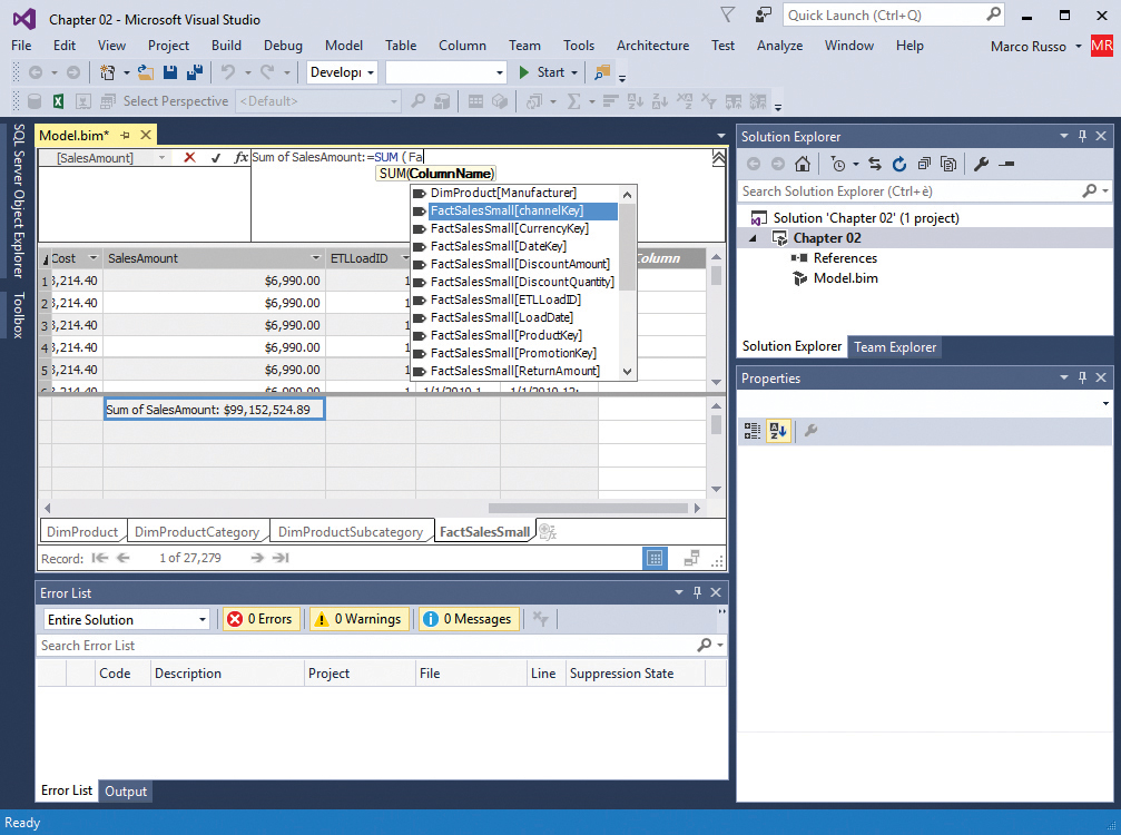
1. In the model you have just created, select the SalesAmount column in the FactSalesSmall table.

2. Click the Sum button. Alternatively, click the drop-down arrow next to the Sum button and choose Sum from the menu that appears, as shown in Figure 2-23.

3. The new measure appears in the measure grid underneath the highlighted column, as shown in Figure 2-24. When a measure is selected in the measure grid, its properties are displayed in the Properties pane. The measure name and a sample output (which is the aggregated total of the rows that are currently being displayed) are shown in the measure grid. Click the cell that contains the measure name and sample output to display the DAX definition of the measure in the formula bar. There, it can be edited.

4. Repeat steps 1–3 for the TotalCost column. You now have two measures in the data model.

5. By default, a measure appears in the measure grid underneath the column that was selected when it was created. Its position in the measure grid is irrelevant, however. You can move it somewhere else if you want to. To move a measure in the measure grid, right-click it, choose Cut, select the cell to which you want to move it, and choose Paste.

6. To help you write your own DAX expressions in the formula bar, Visual Studio offers extensive IntelliSense for tables, columns, and functions. As you type, SSDT displays a list of all the objects and functions available in the current context in a drop-down list underneath the formula bar, as shown in Figure 2-25. Select an item in the list and then press Tab to insert that object or function into your expression in the formula bar.

1. Scroll to the far right of the table and click Add Column, as shown in Figure 2-26.

2. Enter a new DAX expression for that column in the formula bar in the following format and press Enter. (Note that IntelliSense works the same way for calculated columns as it does for measures.)

= <scalar DAX expression>

3. A new calculated column is created with a name such as CalculatedColumn1. To rename the calculated column to something more meaningful, double-click the column header and type the new name. Alternatively, edit the value for the Column Name property in the Properties pane on the right.

The second method is as follows:

1. Right-click an existing column and select Insert Column from the menu that appears. This creates a new calculated column next to the column you have just selected.

Before moving on to the next section, follow these steps:

1. In your model, create a new calculated column called Margin, with the following definition:

Click here to view code image

= FactSalesSmall[SalesAmount] - FactSalesSmall[TotalCost]

2. Create a new measure from it by using the Sum button in the same way you did in the previous section.

= <table DAX expression>

You specify a DAX expression returning a table, which is evaluated and stored when you refresh the data model. This is similar to what you do for a calculated column. The only difference is that you must specify an expression that generates columns and rows of the table you want to store in the model. A new calculated table is created, with a name such as CalculatedTable1. You can give it a more meaningful name by either double-clicking the name in the table tabs and entering the new name or editing the Table Name property in the Properties pane. For example, you can create a table named Dates containing all the dates required for the fact table by using the following definition, obtaining the result shown in Figure 2-27:

Click here to view code image

= ADDCOLUMNS (
    CALENDARAUTO(),
    "Year", YEAR ( [Date] ),
    "Month", FORMAT ( [Date], "MMM yyyy" ),
    "MonthNumber", YEAR ( [Date] ) * 100 + MONTH ( [Date] )
)

In the diagram view, you can opt to display all the tables in your model or only the tables that are present in a particular perspective. You can also choose whether to display all the object types or just the columns, measures, hierarchies, or KPIs associated with a table by selecting and clearing the boxes in the Display pop-up menu at the bottom of the pane. You can automatically arrange the tables in the model by clicking the Reset Layout button, by arranging all the tables so they fit on one screen (by clicking the Fit to Screen button), and by zooming in and out (by dragging the slider at bottom edge of the pane). In the diagram view, you can rearrange tables manually by dragging and dropping them if you click and drag their blue table header bars. You can resize a table by clicking its bottom-left corner, and you can maximize a table so that all the columns in the table are displayed by clicking the Maximize button in the right corner of the table header bar. Each of these interface elements is shown in Figure 2-28.

After a relationship has been created, you can delete it by clicking it to select it and pressing the Delete key. You can also edit it by double-clicking it or by selecting Manage Relationships from the Table menu. This displays the Manage Relationships dialog box, shown in Figure 2-29. There, you can select a relationship for editing. This displays the Edit Relationship dialog box (also shown in Figure 2-29).

The model you have been building should already have the following relationships:

Between FactSalesSmall and DimProduct, based on the ProductKey column.

Between DimProduct and DimProductSubcategory, based on the ProductSubcategoryKey column.

Between DimProductSubcategory and DimProductCategory, based on the ProductCategoryKey column.

These relationships were created automatically because they were present as foreign key constraints in the SQL Server database. If they do not exist in your model, create them now.

The Edit Relationship dialog box shows the following additional information about the relationship that you will see in more detail in Chapter 6:

Cardinality This can be Many to One (*:1), One to Many (1:*), or One to One (1:1).

Filter Direction This can have a single direction (from the table on the One side to the table on the Many side of a relationship) or can be bidirectional (the filter propagates to both tables).

Active You can enable this on only one relationship connecting two tables in case more than one relationship’s path connects two tables.

The table named Dates that you created before (as a calculated table) does not have any relationship with other tables until you explicitly create one. For example, by clicking Create Relationship from the Table menu, you can create a relationship between the FactSalesSmall and Dates tables using the DateKey column of the FactSalesSmall table and the Date column of the Dates table, as shown in Figure 2-30.

1. Select the DimProduct table and click the Maximize button so that as many columns as possible are visible.

2. Click the Create Hierarchy button on the table.

3. A new hierarchy will be created at the bottom of the list of columns. Name it Product by Color.

4. Drag the ColorName column down onto it to create the top level. (If you drag it to a point after the hierarchy, nothing will happen, so be accurate.)

5. Drag the ProductName column below the new ColorName level to create the bottom level, as shown in Figure 2-31.

6. Click the Restore button (which is in the same place the Maximize button was) to restore the table to its original size.

You can enter text in the Search box in the Tabular Model Explorer pane to quickly locate any entity in the data model that includes the text you typed. For example, Figure 2-33 shows only the entities containing the word Sales in any part of the name. You can see the measures, relationships, tables, columns, and partitions that include the word Sales in their name.

1. Open the Build menu and click Deploy. The metadata for the database is deployed to your development server. Then it is processed automatically if you have left the project’s Processing Option property set to Default.

2. If you chose to use a Windows user name on the Impersonation Information screen of the Table Import wizard for creating your data source, you might need to reenter the password for your user name at this point. After processing has completed successfully, you should see a large green check mark with the word Success, as shown in Figure 2-34.

The model is now present on your development server and ready to be queried.

This section focuses on Excel 2016 as a client tool. End users can use an earlier version of Excel, but it will not have the same functionality. Excel versions from 2007 to 2013 are very similar to Excel 2016, but Excel 2003 and earlier versions provide only basic support for querying Analysis Services and have not been fully tested with Analysis Services tabular models.

1. Open the Model menu and click Analyze in Excel. (There is also a button on the toolbar with an Excel icon on it that does the same thing.) This opens the Analyze in Excel dialog box, shown in Figure 2-35.

2. Choose one of the following options:

• Current Windows User This is the default setting. It enables you to connect to your workspace database as yourself and see all the data in there.

• Other Windows User or Role These settings enable you to connect to the database as if you were another user to test security. They are discussed in more detail in Chapter 10, “Security.”

• Perspective This option enables you to connect to a perspective instead of the complete model.

• Culture This option allows you to connect using a different locale setting, displaying data in a different language if the model includes translations. Translations are discussed in Chapter 8.

3. Click OK. Excel opens and a blank PivotTable connected to your database is created on the first worksheet in the workbook, as shown in Figure 2-36.

1. Start Excel.

2. Click the Data tab on the ribbon and click the From Other Sources button in the Get External Data group.

3. Select From Analysis Services, as shown in Figure 2-37.

4. This starts the Data Connection wizard. On the first page, enter the name of the instance of Analysis Services to which you wish to connect and click Next. (Do not change the default selection of Use Windows Authentication for logon credentials.)

5. Choose the database to which you want to connect and the cube you want to query. (If you are connecting to a workspace database, you will probably see one or more workspace databases with long names incorporating globally unique identifiers, or GUIDS.) There are no cubes in a tabular database, but because Excel predates the tabular model and generates only MDX queries, it will see your model as a cube. Therefore, choose the item on the list that represents your model, which, by default, will be called Model, as shown in Figure 2-38. If you defined perspectives in your model, every perspective will be listed as a cube name in the same list.

6. Click Next.

7. Click Finish to save the connection and close the wizard.

8. You will be asked whether you want to create a new PivotTable, a new PivotChart, a new Power View report, or just a connection. If you are creating a PivotTable, you must also choose where to put it. Create a new PivotTable and click OK to return to the point shown back in Figure 2-36.

You can select measures either by choosing them in the PivotTable Fields pane or dragging them down into the Values area in the bottom-right corner of the PivotTable Fields pane. In a similar way, you can select columns either by clicking them or by dragging them to the Columns, Rows, or Filters areas in the bottom half of the PivotTable Fields pane. Columns and hierarchies become rows and columns in the PivotTable, whereas measures display the numeric values inside the body of the PivotTable. By default, the list of measures you have selected is displayed on the columns axis of the PivotTable, but it can be moved to rows by dragging the Values icon from the Columns area to the Rows area. You cannot move it to the Filters area, however. Figure 2-39 shows a PivotTable using the sample model you have built with two measures on columns, the Product by Color hierarchy on rows, and the ProductCategoryName field on the filter.

1. From the Insert tab on the ribbon, click the Slicer button in the Filters group.

2. In the Insert Slicers dialog box, select the field you want to use, as shown in Figure 2-40, and click OK. The slicer is added to your worksheet.

After the slicer is created, you can drag it wherever you want in the worksheet. You then only need to click one or more names in the slicer to filter your PivotTable. You can remove all filters by clicking the Clear Filter button in the top-right corner of the slicer. Figure 2-41 shows the same PivotTable as Figure 2-40 but with the filter ProductCategoryName replaced by a slicer and with an extra slicer added, based on ProductSubcategoryName.

When there are multiple slicers, you might notice that some of the items in a slicer are shaded. This is because, based on the selections made in other slicers, no data would be returned in the PivotTable if you selected the shaded items. For example, in Figure 2-41, on the left side, the TV And Video item on the ProductCategoryName slicer is grayed out. This is because no data exists for that category in the current filter active in the PivotTable above the slicers, which includes only Pink, Red, and Transparent as possible product colors. (Such a selection is applied straight to the product colors visible on the rows of the PivotTable.) In the ProductSubcategoryName slicer, all the items except Cell Phones Accessories and Smart Phones & PDAs are shaded because these are the only two subcategories in the Cell Phones category (which is selected in the ProductCategoryName slicer on the left) for the product colors selected in the PivotTable.

Putting an attribute on a slicer enables you to use it on rows, on columns, or in the Filter area of the PivotTable. This is not the case of an attribute placed in the Filter area, which cannot be used on rows and columns of the same PivotTable. You can also connect a single slicer to many PivotTables so that the selections you make in it are applied to all those PivotTables simultaneously.

When you click any field in the PivotTable Fields list or in the drop-down arrow next to the Row Labels or Column Labels box in the PivotTable, you can choose individual items to display and apply sorting and filtering, as shown in Figure 2-42.

Selecting and clearing members in the list at the bottom of the dialog box selects and clears members from the PivotTable. It is also possible to filter by the names of the items and by the value of a measure by using the Label Filters and Value Filters options.

If you need more control over which members are displayed and in which order they are shown, you must use a named set. To create a named set, follow these steps:

1. Click the Analyze tab in the PivotTable Tools section on the ribbon.

2. In the Calculations group, click Fields, Items, & Sets and select either Create Set Based on Row Items or Create Set Based on Column Items, as shown in Figure 2-43.

3. The New Set dialog box then appears, as shown in Figure 2-44. Here, you can add, delete, and move individual rows in the PivotTable. If you have some knowledge of MDX, click the Edit MDX button (in the lower-right portion of the dialog box) and write your own MDX set expression to use.

4. Click OK to create a new named set.

You can think of a named set as being a predefined selection that is saved with the PivotTable, but does not necessarily need to be used. After you create the named set, it appears under a folder called Sets in the PivotTable Fields list, as shown in Figure 2-45. As long as you leave the Replace the Fields Currently in The Row/Column Area with the New Set option selected in the bottom of the New Set dialog box (refer to Figure 2-44), your set will control what appears on the rows in the PivotTable.

1. Click the Analyze tab on the PivotTables Tools section of the ribbon.

2. Click the OLAP Tools button in the Calculations group and select Convert to Formulas from the drop-down menu, as shown in Figure 2-46. The result is also shown in Figure 2-46.

Notice how in Figure 2-46 the B2 cell returns the value of the measure Sum of SalesAmount for pink products, but this value is returned now by the following formula:

Click here to view code image

=CUBEVALUE("localhost_Tabular Chapter 02_marco_42571bd5-ef40-440f-b3f6-a7cb5270b027",$A2,B$1,
Slicer_ProductCategoryName)

The four parameters used in the CubeValue() function here are as follows:

The name of the Excel connection to Analysis Services

A cell reference to cell A2, which contains another function that returns the item name Pink

Another cell reference to cell B1, which returns the measure Sum of SalesAmount

A reference to the slicer containing the product category names

As a result, this cell returns the value from the cube for the Sum of SalesAmount, Pink products, and the product category Cell Phones.

Cube formulas are a very powerful way of displaying free-form reports in Excel and allow much greater flexibility in layout and formatting than PivotTables. Their one drawback is that they do not allow as much interactivity as PivotTables. Users can no longer change what appears on rows and columns by dragging and dropping, nor can they navigate down through hierarchies (although slicers and report filters still work as expected).

It is beyond the scope of this book to provide a full description of what Excel cube formulas can do. If you would to learn more about them, Excel help, found at https://support.office.com/en-us/article/Cube-functions-reference-2378132b-d3f2-4af1-896d-48a9ee840eb2, is a good place to start.

1. Open Power BI Desktop.

2. In the Home tab’s External Data group on the ribbon, click the Get Data drop-down arrow and select Analysis Services, as shown in Figure 2-47.

3. The SQL Server Analysis Services Database opens. Enter the server name corresponding to the tabular instance of Analysis Services (see Figure 2-48).

4. Select the Connect Live option button, as shown in Figure 2-48, to create a report that interactively queries Analysis Services. Then click OK.

5. The Navigator dialog box opens, displaying a list of the databases available in the Analysis Services. For each one, you can see the models and perspectives available. As shown in Figure 2-49, choose the model (named Model) in the Chapter 02 database. Then click OK.

To add a table to the report, follow these steps:

1. Drag the ProductCategoryName column from the DimProductCategory table into the Values area in the Visualizations pane.

2. Repeat step 1 with the ProductSubcategoryName column from the DimProductSubcategory table.

3. Repeat step 1 with the Sum of SalesAmount measure defined in the FactSalesSmall table. This creates a new table in the report page.

4. Resize the table by clicking the bottom-left edge and expanding it, so all the data is visible. The result should look like the report shown in Figure 2-51.

1. Click somewhere inside the table.

2. In the Visualizations pane, select a chart type, such as a Stacked Bar Chart.

You can add a slicer inside the page to provide another way of filtering the chart you have just created. Follow these steps:

1. Drag the Color column from the DimProduct table into the empty space to the right of the chart to create a new table.

2. Click inside the table.

3. In the Visualizations pane, click the Slicer button (the bottom-left corner icon in the Visualizations pane) to turn the table into a slicer.

In addition to resizing the controls, you can also move them around to improve the layout of the view by hovering over the top-right side of a control until the mouse turns into a figure icon and then dragging it. Selecting a color name inside the slicer filters the values that are used in the chart.

One of the coolest visualizations available in Power BI is the animated scatter chart. To create one on your report, follow these steps:

1. Click the empty space at the bottom of the report.

2. Click the Scatter Chart button in the Visualizations pane (the third row down on the far left).

3. Assign to each visualization property the following columns or measures (you can use drag and drop to do this):

• Details Drag the ProductSubcategoryName column from the DimProductSubcategory table.

• Legend Drag the ProductCategoryName column from the DimProductCategory table.

• X Axis Drag the UnitPrice column from the FactSalesSmall table. Then click the drop-down arrow next to it and select Average. This creates a new measure just for this report that returns the average price of sales transactions.

• Y Axis Drag the SalesQuantity column from the FactSalesSmall table. This creates a new measure just for this report that returns the sum of the quantity in sales.

• Size Drag the sum of the SalesAmount measure from the FactSalesSmall table.

• Play Axis Drag the MonthNumber column from the Dates table.

4. The report should now look like the one shown in Figure 2-52. To save the report, open the File menu and choose Save.

1. Click the up-arrow button in the top-right corner of the ribbon, next to the Help button, to minimize the ribbon.

2. The scatter chart still does not have much space. To make more room for it, click the Focus Mode button in the top-right corner of the chart to expand it to the full screen, as shown in Figure 2-53.

3. Click the Play button in the bottom-left corner to show an animation of how the sales of the product categories, their order volumes, and their average product costs change over time.

4. To return the scatter chart to its original size, again click the Focus Mode button in the top-right corner of the report.

In the Filters area of the Visualizations pane, you can apply filters to individual charts, individual pages or the whole report. In Figure 2-53 you can see a filter of three product categories applied to the scatter chart visualization only.

1. Open SSMS.

2. In the Connect to Server dialog box that appears, choose Analysis Services in the Server Type drop-down box.

3. Enter your instance name in the Server Name box, as shown in Figure 2-54.

4. Click Connect.

5. A new connection to Analysis Services opens in the Object Explorer pane. Expand all the available nodes on a tabular instance to see something similar to what is displayed in Figure 2-55, which shows the database you created and deployed earlier in this chapter.

At the top of the pane is the Instance node, showing the name of the instance, the version number, and your user name. Underneath that is a folder containing a list of databases. Inside each database, you can see the connections, tables, and security roles inside that database. Right-clicking any of these objects enables you to view and edit their properties. In the case of the instance, this is the only place in which Analysis Services server properties can be edited in a user interface. In addition, you can process databases and individual tables, and you can script out objects to XMLA or JSON. All this functionality is covered in more detail in Chapter 11, “Processing and partitioning tabular models,” and in Chapter 13, “Interfacing with Tabular.”

It is also possible to execute both DAX and MDX queries against a tabular model in SSMS. Although confusing, both must be executed through an MDX query pane. To open one, you can do one of the following:

Click the New MDX Query button on the toolbar The same Connect to Server dialog box appears as when you opened a connection in Object Explorer.

Right-click a database in the Object Explorer pane, select New Query, and choose MDX You will be connected directly to the database you have clicked, but you can change the database to which you are connected by using the Database drop-down box in the toolbar.

After you have connected, your new MDX query pane appears, where you can enter your MDX or DAX query (see Figure 2-56).

To run the query, click the Execute button on the toolbar or press F5. To cancel a query during execution, click the red Cancel button next to the Execute button. You can try this yourself by running the following DAX query against the model you have built, which returns the DimProductCategory table:

EVALUATE DimProductCategory

The subject of writing DAX queries is part of the larger topic of the DAX language, which is introduced in Chapter 4. Detailed coverage of DAX is available in The Definitive Guide to DAX, written by the authors of this book and published by Microsoft Press.

Like what happens when you create a new tabular project in SSDT by starting from a Power Pivot model, if the service account running Analysis Services does not have read permissions on the data sources, you might have to modify the security settings in the connection properties of the imported database. You can do this using the corresponding feature in SSMS.

As you see in Figure 2-58, its layout is similar to SSMS. It also allows the execution of MDX and DAX queries, but it provides features that help the DAX syntax only. The Metadata pane shows tables, columns, and measures of the database and perspective selected in the drop-down lists above. Clicking the Run button on the toolbar or pressing F5 executes the query, and you can cancel a running execution by clicking the Cancel button in the ribbon. DAX Studio also offers an integrated environment to analyze the query plan and the timings of the internal operations that are executed within a query, without having to open SQL Profiler to capture such events.