Chapter 5. Building hierarchies
Hierarchies are a much more important part of a tabular model than you might think. Even though a tabular model can be built without any hierarchies, hierarchies add a lot to the usability of a model—and usability issues often determine the success or failure of a business intelligence (BI) project. The basic process of building a hierarchy was covered in Chapter 2, “Getting started with the tabular model.” This chapter looks at the process in more detail and discusses some of the more advanced aspects of creating hierarchies: when you should build them, what the benefits and disadvantages of using them are, how you can build ragged hierarchies, and how you can model parent-child relationships.
![]() What’s new in SSAS 2016
What’s new in SSAS 2016
This chapter describes features that were already present in previous versions. SSAS 2016 does not provide new features in this area.
Basic hierarchies
First, we will look at what a hierarchy is and how to build basic hierarchies.
What are hierarchies?
By now, you are very familiar with the way a tabular model appears to a user in a front-end tool, such as Microsoft Excel, and the way the distinct values in each column in your model can be displayed on the rows or columns of a Microsoft Excel PivotTable. This provides a very flexible way of building queries, but it has the disadvantage that every new level of nesting that you add to the row or column axis requires a certain amount of effort for the user. First, the user must find what he or she wants to add and then click and drag it to where it should appear. More importantly, it requires the user to have a basic level of understanding of the data he or she is using. To build meaningful reports, the user must know information—such as the fact that a fiscal semester contains many fiscal quarters, but a fiscal quarter can be in only one fiscal semester—so that he or she can order these items appropriately on an axis.
Hierarchies provide a solution to these problems. You can think of them as predefined pathways through your data that help your users explore down from one level of granularity to another in a meaningful way. A typical example of a hierarchy would be on a Date table, in which users often start to view data at the Year level and then navigate down to Quarter, Month, and Date level. A hierarchy enables you to define this type of navigation path. Figure 5-1 shows what a hierarchy looks like when used in an Excel PivotTable.

A hierarchy like this can save your users time by helping them find what they are looking for quickly. With a hierarchy, there is only one thing to drag and drop into a PivotTable, after which users just double-click an item to drill down until they get to the level of detail they require.
Hierarchies can also prevent users from running queries that return more data than they want and that might perform badly. For example, a user might drag every date in the Date table onto the rows of a PivotTable and then filter those rows to show just the ones in which the user is interested, which would be slow because displaying every date could result in a query that returns hundreds of rows. Instead, a hierarchy encourages the user to choose a year, navigate to display just the quarters in that year, and then navigate until he or she reaches the date level, which results in much smaller, faster queries at each step.
![]() Note
Note
Microsoft Power BI recognizes hierarchies defined in a tabular model, and it uses them to enable drill-down navigation across hierarchies’ levels. However, Power View in Excel 2013/2016 does not have this capability, so Power View users cannot take advantage of this feature.
When to build hierarchies
There are several advantages to building hierarchies. That does not mean you should build hundreds of them on every table, however. The following guidelines explain when to build hierarchies and when not to:
![]() You should build hierarchies when one-to-many relationships exist between the columns in a single table because this usually indicates the existence of an underlying pattern in the data itself. Often, these patterns represent a natural way for users to explore the data. A hierarchy going from Year to Quarter to Month to Date has already been described; other common examples include hierarchies going from Country to State to City to ZIP Code to Customer, or from Product Category to Product Subcategory to Product.
You should build hierarchies when one-to-many relationships exist between the columns in a single table because this usually indicates the existence of an underlying pattern in the data itself. Often, these patterns represent a natural way for users to explore the data. A hierarchy going from Year to Quarter to Month to Date has already been described; other common examples include hierarchies going from Country to State to City to ZIP Code to Customer, or from Product Category to Product Subcategory to Product.
![]() You can build hierarchies when one-to-many relationships do not exist between columns, but when certain columns are frequently grouped together in reports. For example, a retailer might want to drill down from Product Category to Brand to Style to Color to Product, even if there is a many-to-many relationship among Brand, Style, and Color. Just consider possible performance issues for unnatural hierarchies when using certain versions of Excel as a client, as described later in this chapter.
You can build hierarchies when one-to-many relationships do not exist between columns, but when certain columns are frequently grouped together in reports. For example, a retailer might want to drill down from Product Category to Brand to Style to Color to Product, even if there is a many-to-many relationship among Brand, Style, and Color. Just consider possible performance issues for unnatural hierarchies when using certain versions of Excel as a client, as described later in this chapter.
![]() Hierarchies tend to be more useful the more levels they have. There is no point in building a hierarchy with just one level in it, and hierarchies with two levels might not provide much benefit.
Hierarchies tend to be more useful the more levels they have. There is no point in building a hierarchy with just one level in it, and hierarchies with two levels might not provide much benefit.
You can make hierarchies visible to perspectives and choose whether attributes used in hierarchies are visible for each perspective. As you will see in the “Hierarchy design best practices” section later in this chapter, you can force users to use only a hierarchy instead of its underlying columns by hiding those columns.
With the ease of use that hierarchies bring comes rigidity. If you have defined a hierarchy that goes from Product Category to Brand, and if the underlying columns are hidden, Excel users will not be able to define a report that places Brand before Product Category, nor will they be able to place Product Category and Brand on opposing axes in a report. However, other clients, such as Power BI, are more flexible and allow for the selection of data from a single level of a hierarchy, without having to previously filter higher hierarchical levels.
Building hierarchies
There are essentially two steps involved in creating a hierarchy:
1. Prepare your data appropriately.
2. Build the hierarchy on your table.
You can perform the initial data-preparation step inside the tabular model itself. This chapter discusses numerous techniques to do this. The main advantages of doing your data preparation inside the tabular model are that, as a developer, you need not switch between several tools when building a hierarchy, and you have the power of DAX at your disposal. This might make it easier and faster to write the logic involved. However, whenever possible, you should consider preparing data inside your extract, transform, load (ETL) process. You can do this either in a view or in the SQL code used to load data into the tables in your tabular model. The advantage of this approach is that it keeps relational logic in the relational database, which is better for maintainability and reuse. It also reduces the number of columns in your model and improves the compression rate so that your model has a smaller memory footprint. Additionally, if you are more comfortable writing SQL than DAX, it might be easier from an implementation point of view.
You design hierarchies in SQL Server Data Tools (SSDT) in the diagram view. To create a hierarchy on a table (it is not possible to build a hierarchy that spans more than one table), do one of the following:
![]() Click the Create Hierarchy button in the top-right corner of the table.
Click the Create Hierarchy button in the top-right corner of the table.
![]() Select one or more columns in the table, right-click them, and select Create Hierarchy to use those columns as the levels in a new hierarchy.
Select one or more columns in the table, right-click them, and select Create Hierarchy to use those columns as the levels in a new hierarchy.
To add a new level to an existing hierarchy, do one of the following:
![]() Drag and drop a column into it at the appropriate position.
Drag and drop a column into it at the appropriate position.
![]() Right-click the column, select Add to Hierarchy, and click the name of the hierarchy to which you wish to add it.
Right-click the column, select Add to Hierarchy, and click the name of the hierarchy to which you wish to add it.
After a hierarchy has been created, you can move the levels in it up or down or delete them by right-clicking them and choosing the desired option from the context menu that appears. To rename a hierarchy, double-click its name, or right-click its name and choose Rename from the context menu.
You can create any number of hierarchies within a single table. Figure 5-2 shows what a dimension with multiple hierarchies created in SSDT looks like.

Hierarchy design best practices
Consider the following tips when designing hierarchies:
![]() After you include a column from a table as a level in a hierarchy, you can hide the column itself by right-clicking it and selecting Hide from Client Tools. It is then visible only to your users as a level in a hierarchy. This is usually a good idea because it stops users from becoming confused about whether they should use the original column or the hierarchy in their reports or whether there is any difference between the column and the hierarchy. Users then also have a shorter list of items to search when building their reports, making it easier to find what they want. However, in some client tools, it can make filtering on values that make up lower levels of the hierarchy (such as Month in the hierarchy shown previously in Figure 5-2) much harder.
After you include a column from a table as a level in a hierarchy, you can hide the column itself by right-clicking it and selecting Hide from Client Tools. It is then visible only to your users as a level in a hierarchy. This is usually a good idea because it stops users from becoming confused about whether they should use the original column or the hierarchy in their reports or whether there is any difference between the column and the hierarchy. Users then also have a shorter list of items to search when building their reports, making it easier to find what they want. However, in some client tools, it can make filtering on values that make up lower levels of the hierarchy (such as Month in the hierarchy shown previously in Figure 5-2) much harder.
![]() Levels in different hierarchies should not have the same name if they represent different things. For example, if you have Fiscal and Calendar hierarchies on your Date dimension, the top levels should be Fiscal Year and Calendar Year, respectively, and neither should be named Year. This removes a possible cause of confusion for your users.
Levels in different hierarchies should not have the same name if they represent different things. For example, if you have Fiscal and Calendar hierarchies on your Date dimension, the top levels should be Fiscal Year and Calendar Year, respectively, and neither should be named Year. This removes a possible cause of confusion for your users.
![]() It can be a good idea to follow a standard naming convention for hierarchies to help your users understand what they contain. For example, you might have a hierarchy that goes from Year to Quarter to Month to Date and another that goes from Year to Week to Date. Calling the first hierarchy Year-Month-Date and the second one Year-Week-Date would make it easier for your users to find the one they need in their front-end tool.
It can be a good idea to follow a standard naming convention for hierarchies to help your users understand what they contain. For example, you might have a hierarchy that goes from Year to Quarter to Month to Date and another that goes from Year to Week to Date. Calling the first hierarchy Year-Month-Date and the second one Year-Week-Date would make it easier for your users to find the one they need in their front-end tool.
Hierarchies spanning multiple tables
Even if it is not possible to create hierarchies that span multiple tables, you might find yourself needing to do this if you have snowflaked dimension tables. One solution is to denormalize the dimension tables in the relational data source—for example, in a view. You can achieve the same effect relatively easily by using calculated columns.
The Product dimension in the Contoso DW sample database is a good example of a snowflaked dimension. It is made up of three tables that we imported into the data model (Product Category, Product Subcategory, and Product), as shown in Figure 5-3.

It is possible that, given a dimension like this, users would want to drill down from Product Category to Product Subcategory to Product. To enable this, you must first bring the names of the subcategory and category for each product down to the Product table by creating two calculated columns there. The DAX formulas required for this are fairly simple:
Product[Subcategory] = RELATED ( 'Product Subcategory'[Subcategory] )
Product[Category] = RELATED ( 'Product Category'[Category] )
Figure 5-4 shows what these two new calculated columns look like in the Product table.

You can then create a hierarchy on the Product table that goes from Category to Subcategory to Product, as shown in Figure 5-5. As a final step, it is advisable to completely hide the Product Category and Product Subcategory tables (right-click them and select Hide from Client Tools) because the new hierarchy removes the need to use any of the columns on them.

Readers familiar with multidimensional models might know that it is possible to create ragged hierarchies in them, in which the user skips a level in a hierarchy in certain circumstances. One example of when this is useful is a Geography hierarchy that goes from Country to State to City, but in which the user can drill down from Country directly to City for countries that are not subdivided into states. Another example is when leaf members exist on different levels of a hierarchy.
The tabular model does not support this functionality in the model compatibility level 1200. In previous versions, it was possible to create ragged hierarchies in SSDT, leveraging the HideMemberIf property exposed by BIDS Helper. However, this was an unsupported feature, and it only worked using Excel as a client. We hope Microsoft provides a native implementation of ragged hierarchies in Tabular in a future update.
Natural and unnatural hierarchies
A hierarchy in a tabular model does not have any performance impact on DAX queries. This is mainly because DAX offers no way to reference a hierarchy. However, different types of hierarchies may generate different MDX queries and different corresponding query plans. In particular, there are differences between natural and unnatural hierarchies, which you will see shortly.
![]() Note
Note
The issue described in this section does not affect a PivotTable in Excel 2016 that queries a tabular model hosted on Analysis Services 2016. However, different combinations of older versions are subject to memory and performance issues, when an MDX query includes unnatural hierarchies.
A natural hierarchy has a single parent for each unique value of a level of the hierarchy. When this is not true, then the hierarchy is said to be unnatural. For example, the hierarchy you saw at the beginning of this chapter, in Figure 5-1, is a natural hierarchy because every month has 12 unique values for each year, so each month has only one parent. In practice, the name is not just the month name, but is a combination of both the month name and year. In this way, the value is unique across all the branches of the hierarchy. In a multidimensional model, you can define attribute relationships, which enforces the existence of a natural hierarchy. You also get an error during processing in case the data does not respect the constraints defined. However, there is no similar setting in Tabular. Based on data coming from the data source, the engine automatically marks a hierarchy as natural or unnatural.
For example, Figure 5-6 shows an example of unnatural hierarchy. In this case, the month name does not include the year, so the value of March can have multiple parents: CY 2007, CY 2008, and other years that are not visible in the screenshot.

If you want to support previous versions of Excel and Analysis Services, you should consider creating only natural hierarchies. For more details on performance issues caused by unnatural hierarchies, see http://www.sqlbi.com/articles/natural-hierarchies-in-power-pivot-and-tabular/.
Parent-child hierarchies
Now that you have seen how to create a basic hierarchy, you can consider how to manage parent-child hierarchies, which require a specific data preparation.
What are parent-child hierarchies?
In dimensional modeling, a parent-child hierarchy is a hierarchy in which the structure is defined by a self-join on a dimension table rather than by modeling each level as a separate column, as in a regular dimension. Typical scenarios in which you might use a parent-child hierarchy include the organizational structure of a company or a chart of accounts. The main advantage of this way of modeling a dimension is that you do not need to know the maximum depth of the hierarchy at design time. If, for example, your company undergoes a reorganization, and there are suddenly 20 steps in the chain of command—from the lowliest employee up to the CEO—when previously there were only 10, you do not need to change your dimension table. Figure 5-7 shows the original Employee table from the Contoso DW sample database. (The table is imported through a view in the data model, as you can see in the examples in the companion content.)

In Figure 5-7, the primary key of the table is the EmployeeKey column, and each row represents an individual employee of the Contoso corporation. The employees’ names are held in the Name column. The ParentEmployeeKey column holds the value of the EmployeeKey column for the employee’s manager.
Configuring parent-child hierarchies
After all this explanation, it might come as something of a letdown to discover that, unlike the multidimensional model, the tabular model does not support true parent-child hierarchies. However, it does have some very useful DAX functionality for flattening parent-child hierarchies into regular, column-based hierarchies. This is good enough for most scenarios, although it means that you have to make an educated guess at design time about what the maximum depth of your hierarchy will be. In this section, you learn how to configure a simple parent-child hierarchy by using the Employee table as an example. You also find out how to handle more complex design problems.
Building a basic parent-child hierarchy
The first step in building a hierarchy on the Employee table is to create a calculated column that contains the list of values for EmployeeKey from the top of the hierarchy down to the current employee. To do this, create a calculated column called EmployeePath and use the following DAX expression:
Employee[EmployeePath] =
PATH ( Employee[EmployeeKey], Employee[ParentEmployeeKey] )
The output of the PATH function is a pipe-delimited list of values, as shown in Figure 5-8. (If your key column contains pipe characters, you might have some extra data cleaning work to do.)

You can use the contents of this column to create more calculated columns to represent each level in your hierarchy. Before you do that, though, you need to know how many levels you must create. You can do this by creating one more calculated column, called HierarchyDepth, that returns the number of items in the list returned in the EmployeePath column. To do so, use the following PATHLENGTH function:
Employee[HierarchyDepth] =
PATHLENGTH ( Employee[EmployeePath] )
You can then build a measure to return the maximum value in this column by using the following definition:
[Max Depth] :=
MAX ( Employee[HierarchyDepth] )
In the case of the Employee table, the maximum depth of the hierarchy is four levels, so you must create at least four new calculated columns for the levels of your new hierarchy. However, as mentioned, it might be wise to build some extra levels in case the hierarchy grows deeper over time.
To populate these new calculated columns, you must find the employee name associated with each key value in the path returned in the EmployeePath calculated column. To find the key value at each position in the path contained in the EmployeePath column, you can use the PATHITEM function, as follows:
PATHITEM ( Employee[EmployeePath], 1, INTEGER )
There are three parameters to the PATHITEM function. The first parameter takes the name of the column that contains the path. The second parameter contains the 1-based position in the path for which you want to return the value. The third parameter, which is optional, can be either TEXT (which means the value will be returned as text) or INTEGER (which means the value will be returned as an integer). You can also use 0 for TEXT and 1 for INTEGER, although we recommend using the enumeration name to make the formula easier to read.
The third parameter can be important for matching the value returned by PATHITEM with the value in the key column of the table. If you omit the third parameter, it will be returned as TEXT by default. In this case, however, if the value has to be compared with an integer (as in the example shown here), then the conversion from text to integer will be made implicitly at the moment of the comparison. In any case, the three following syntaxes are equivalent:
PATHITEM ( Employee[EmployeePath], 1, INTEGER )
INT ( PATHITEM ( Employee[EmployeePath], 1, TEXT ) )
INT ( PATHITEM ( Employee[EmployeePath], 1 ) )
You can make this conversion automatically when you make a comparison of this value with another value, such as when using LOOKUPVALUE. Thus, it is important to specify the third parameter only when you want to store the result of PATHITEM in a calculated column, which will be created with the data type specified by the value of the third parameter. That said, using the third parameter is a good practice because it shows other developers who might see your code what type of values you are expecting to return.
Key values on their own are not very useful, however. You must find the name of the employee associated with each key. You can do that by using the LOOKUPVALUE function. The following complete expression can be used to return the name of the employee, for the first level in the hierarchy:
Employee[EmployeeLevel1] =
LOOKUPVALUE (
Employee[Name],
Employee[EmployeeKey],
PATHITEM ( Employee[EmployeePath], 1, INTEGER )
)
The following expression is for the second level in the hierarchy:
Employee[EmployeeLevel2] =
LOOKUPVALUE (
Employee[Name],
Employee[EmployeeKey],
PATHITEM ( Employee[EmployeePath], 2, INTEGER )
)
With all four calculated columns created for the four levels of the hierarchy, the table will look like the screenshot in Figure 5-9.

The final step is to create a hierarchy from these columns, in the way you saw earlier in this chapter. In Excel, the result looks like the hierarchy shown in Figure 5-10.
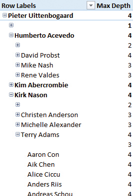
Handling empty items
The approach described in the previous section is sufficient for many parent-child hierarchies. However, as you can see in Figure 5-10, the hierarchy built from the Employee table contains some items that have no name. This is because not all branches of the hierarchy reach the maximum depth of four levels. Rather than show these empty values, it might be better to repeat the name of the member that is immediately above in the hierarchy. You can achieve this by using the IF function. The following example shows what the calculated column expression for the lowest level in the hierarchy looks like with this change:
Employee[EmployeeLevel4] =
VAR CurrentLevel = 4
VAR EmployeePreviousLevel = Employee[EmployeeLevel3]
VAR EmployeeKeyCurrentLevel =
PATHITEM ( Employee[EmployeePath], CurrentLevel, INTEGER )
RETURN
IF (
Employee[HierarchyDepth] < CurrentLevel,
EmployeePreviousLevel,
LOOKUPVALUE ( Employee[Name], Employee[EmployeeKey], EmployeeKeyCurrentLevel )
)
This makes the hierarchy a bit tidier, but it is still not an ideal situation. Instead of empty items, you now have repeating items at the bottom of the hierarchy on which the user can drill down. You can work around this by using the default behavior of tools such as Excel to filter out rows in PivotTables in which all the measures return blank values. If the user has drilled down beyond the bottom of the original hierarchy, all the measures should display a BLANK value.
To find the level in the hierarchy to which the user has drilled down, you can write the following expression to create a measure that uses the ISFILTERED function:
[Current Hierarchy Depth] :=
ISFILTERED ( Employee[EmployeeLevel1] )
+ ISFILTERED ( Employee[EmployeeLevel2] )
+ ISFILTERED ( Employee[EmployeeLevel3] )
+ ISFILTERED ( Employee[EmployeeLevel4] )
The ISFILTERED function returns True if the column it references is used as part of a direct filter. Because a True value is implicitly converted to 1, and assuming the user will not use a single level without traversing the entire hierarchy, by summing the ISFILTERED called for each level, you can add the number of levels displayed in the report for a specific calculation.
The final step is to test whether the currently displayed item is beyond the bottom of the original hierarchy. To do this, you can compare the value returned by the Current Hierarchy Depth measure with the value returned by the Max Depth measure created earlier in this chapter. (In this case, Demo Measure returns 1, but in a real model, it would return some other measure value.) The following expression defines the Demo Measure measure, and Figure 5-11 shows the result.
[Demo Measure] :=
IF ( [Current Hierarchy Depth] > [Max Depth], BLANK(), 1 )

Unary operators
In the multidimensional model, parent-child hierarchies are often used in conjunction with unary operators and custom rollup formulas when building financial applications. Although the tabular model does not include built-in support for unary operators, it is possible to reproduce the functionality to a certain extent in DAX, and you find out how in this section. Unfortunately, it is not possible to re-create custom rollup formulas. The only option is to write extremely long and complicated DAX expressions in measures.
How unary operators work
For full details about how unary operators work in the multidimensional model, see the SQL Server 2016 technical documentation at http://technet.microsoft.com/en-us/library/ms175417.aspx. Each item in the hierarchy can be associated with an operator that controls how the total for that member aggregates up to its parent. In this implementation in DAX, there is support for only the following two unary operators. (MDX in Multidimensional provides a support for more operators.)
![]() + The plus sign means that the value for the current item is added to the aggregate of its siblings (that is, all the items that have the same parent) that occur before the current item, on the same level of the hierarchy.
+ The plus sign means that the value for the current item is added to the aggregate of its siblings (that is, all the items that have the same parent) that occur before the current item, on the same level of the hierarchy.
![]() – The minus sign means that the value for the current item is subtracted from the value of its siblings that occur before the current item, on the same level of the hierarchy.
– The minus sign means that the value for the current item is subtracted from the value of its siblings that occur before the current item, on the same level of the hierarchy.
The DAX for implementing unary operators gets more complex the more of these operators are used in a hierarchy. For the sake of clarity and simplicity, in this section only, the two most common operators used are the plus sign (+), and the minus sign (–). Table 5-1 shows a simple example of how these two operators behave when used in a hierarchy.

In this example, the Sales, Other Income, and Costs items appear as children of the Profit item in the hierarchy. The value of Profit is calculated as follows:
+ [Sales Amount] + [Other Income] - [Costs]
Implementing unary operators by using DAX
The key to implementing unary operator functionality in DAX is to recalculate the value of your measure at each level of the hierarchy rather than calculate it at a low level and aggregate it up. This means the DAX needed can be very complicated. It is a good idea to split the calculation into multiple steps so that it can be debugged more easily. In this example, we will only implement the plus and minus sign operators.
To illustrate how to implement unary operators, you need a dimension with some unary operators on it, such as the Account view in Contoso. Figure 5-12 shows the operators applied to this hierarchy. On the left side, you see that the main logic is to subtract the Expense and Taxation branches from the Income one. All these high-level branches have only the standard plus sign in their children accounts.

The calculation of Profit and Loss Before Tax has to subtract Expense from the Income totals, which are computed by summing all their children accounts. In a similar way, the Profit and Loss After Tax must subtract the Taxation. An example of the final result is shown in Figure 5-13.

The key point is that although each item’s value can be derived from its leaves’ values, the question of whether a leaf value is added or subtracted when aggregating is determined not only by its own unary operator, but also by that of all the items in the hierarchy between it and the item whose value is to be calculated. For example, the value of Selling, General & Administrative Expenses is simply the sum of all the accounts below that, because all of them have a plus sign as a unary operator. However, each of these accounts should be subtracted when aggregated in the Expense account. The same should be done for each upper level where Expense is included (such as Profit and Loss Before Tax and Profit and Loss After Tax). A smart way to obtain this result is to calculate in advance whether the final projection of an account at a certain level will keep their original value, or if it will be subtracted. You can obtain this same result by multiplying the value by –1. Thus, you can calculate for each account whether you have to multiply it by 1 or –1 for each level in the hierarchy. You can add the following calculated columns to the Account table:
Account[Multiplier] =
SWITCH ( Account[Operator], "+", 1, "-", -1, 1 )
Account[SignAtLevel7] =
IF ( Account[HierarchyDepth] = 7, Account[Multiplier] )
Account[SignAtLevel6] =
VAR CurrentLevel = 6
VAR SignAtPreviousLevel = Account[SignAtLevel7]
RETURN
IF (
Account[HierarchyDepth] = CurrentLevel,
Account[Multiplier],
LOOKUPVALUE (
Account[Multiplier],
Account[AccountKey],
PATHITEM ( Account[HierarchyPath], CurrentLevel, INTEGER )
) * SignAtPreviousLevel
)
The calculated column for the other levels (from 1 to 5) only changes something in the first two lines, as shown by the following template:
Account[SignAtLevel<N>] =
VAR CurrentLevel = <N>
VAR SignAtPreviousLevel = Account[SignAtLevel<N+1>]
RETURN ...
As shown in Figure 5-14, the final results of all the SignAtLevelN calculated columns are used to support the final calculation.

The final calculation simply sums the amount of all the underlying accounts that have the same sign aggregating their value at the displayed level. You obtain this by using the PC Amount measure, based on the simple Sum of Amount, as demonstrated in the following example:
Account[Min Depth] :=
MIN ( Account[HierarchyDepth] )
Account[Current Hierarchy Depth] :=
ISFILTERED ( Account[AccountLevel1] )
+ ISFILTERED ( Account[AccountLevel2] )
+ ISFILTERED ( Account[AccountLevel3] )
+ ISFILTERED ( Account[AccountLevel4] )
+ ISFILTERED ( Account[AccountLevel5] )
+ ISFILTERED ( Account[AccountLevel6] )
+ ISFILTERED ( Account[AccountLevel7] )
'Strategy Plan'[Sum of Amount] :=
SUM ( 'Strategy Plan'[Amount] )
'Strategy Plan'[PC Amount] : =
IF (
[Min Depth] >= [Current Hierarchy Depth],
SWITCH (
[Current Hierarchy Depth],
1, SUMX (
VALUES ( Account[SignAtLevel1] ),
Account[SignAtLevel1] * [Sum of Amount]
),
2, SUMX (
VALUES ( Account[SignAtLevel2] ),
Account[SignAtLevel2] * [Sum of Amount]
),
3, SUMX (
VALUES ( Account[SignAtLevel3] ),
Account[SignAtLevel3] * [Sum of Amount]
),
4, SUMX (
VALUES ( Account[SignAtLevel4] ),
Account[SignAtLevel4] * [Sum of Amount]
),
5, SUMX (
VALUES ( Account[SignAtLevel5] ),
Account[SignAtLevel5] * [Sum of Amount]
),
6, SUMX (
VALUES ( Account[SignAtLevel6] ),
Account[SignAtLevel6] * [Sum of Amount]
),
7, SUMX (
VALUES ( Account[SignAtLevel7] ),
Account[SignAtLevel7] * [Sum of Amount]
)
)
)
Summary
This chapter demonstrated how many types of hierarchies can be implemented in the tabular model. Regular hierarchies are important for the usability of your model and can be built very easily. Parent-child hierarchies present more of a problem, but this can be solved with the clever use of DAX in calculated columns and measures.