The translation of the transformation schema into a structure chart is a translation of a network representation of the activities of a task into a hierarchical representation; the result serves as a basis for writing the code. The translation should introduce as little distortion as possible. To guarantee this, first the translation must retain the separation of the management or controlling work of the process from the data transformation work. In the transformation schema, this division is represented by the separation of control transformations from data transformations. Second, we wish to keep separate the essential model work from necessary implementation work such as formatting data structures for input and output. Third, since the transformation schema does not explicitly represent the work of moving data, we wish to keep the portions of the hierarchy that move data separate from the portions that transform data, making the data transformation portions independent of the specifics of the hierarchy and thus reusable. Fourth, we wish to separate data that passes across a common interface into its use by different essential model fragments as rapidly as possible, so that if the structure of the data for one essential model fragment should change then the processing is not inextricably tangled with the processing for other fragments.
In this chapter, we describe techniques for accomplishing this translation with minimum distortion.
The top of the hierarchy in a structure chart is responsible for the controlling decisions of the activity of the task. This is the same role played by the control transformation on the transformation schema; therefore, the basic structure of the control transformation will translate into the upper-level module structure. The data transformations connected to the control transformation will become lower-level modules.
If no control transformation has been allocated to the task, then a controlling module must be invented to manage all of the data transformations. The manager module may then call each of the subordinates, honoring any sequencing specified by the transformation schema. If data produced by a data transformation is required by another data transformation, then the predecessor transformation must produce its data first. On the other hand, if each data transformation is independent, they may be executed in an arbitrary sequence.
If the modeling techniques decribed in Section 4.3 of Chapter 4, Task Modeling, have been applied, each transformation schema will have at most a single control transformation.
It is possible to encode the logic of a control transformation in an ad-hoc manner by constructing code for each transition and using labels to distinguish states. However, the non-sequential nature of the state diagram does not readily match the sequential nature of code, leading to unstructured code which fails to take advantage of the regular structure of the specification. The following code illustrates some of the problems for the state transition diagram shown in Figure 9.1 (from the Cruise Control mechanism described in Appendix A).
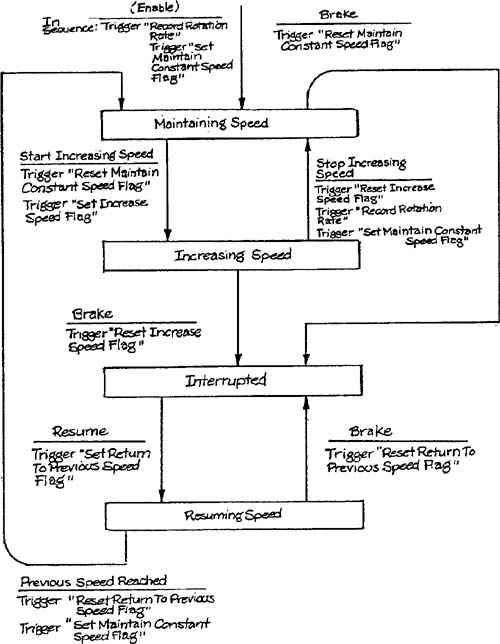
module Control Mode of Operation record rotation rate set maintain constant speed flag maintaining speed: get condition (: condition) if condition = start increasing speed then reset Maintain Constant Speed flag set Increase Speed flag else if condition = brake then reset Maintain Constant Speed flag go to Interrupted else error ("illegal condition", condition:) go to maintaining speed endif endifincreasing speed: get condition (: condition) if condition = stop increasing speed then Reset Increase Speed flags record rotation rate set Maintain Constant Speed flag go to maintaining speed else if condition = brake then reset increase speed flag else error ("illegal condition", condition:) go to increasing speed endif endifinterrupted: get condition (: condition) if condition = resume then set Return to Previous Speed flag else error ("illegal condition", condition :) go to interrupted endifresuming speed: get condition (: condition) if condition = brake then reset Return to Previous Speed flag go to interrupted else if condition = previous speed reached then set Maintain Constant Speed flag reset Return to Previous Speed flag go to maintaining speed else error ("illegal condition", condition:) go to resuming speed endif endifendmodule
The code above makes extensive use of “goto” statements and is therefore likely to be difficult to maintain. Furthermore, the only traces of the state diagram structure are the labels, which have no “enforcement” properties; statements can be inserted at will before or after a label.
In contrast to the code above, there are two more systematic approaches to representing a control transformation on a structure chart: Either the entire transformation (that is, the associated state-transition diagram that specifies it) may be allocated to a single module, or the control transformation may be allocated to several modules — one module per state with a controlling module to select among the submodules. The first strategy requires casting the specification in terms of state transition and action tables as described in Volume 1, Chapter 7, Specifying Control Transformations and shown in Figure 9.2. In Figure 9.2, the actions have been replaced by module names that are called by the controlling module. The code for each of the submodules is simply the actions that were replaced.

The code for the controlling module may now be written as follows:
module Traverse State Tables module ← initial module state ← initial state do forever do action (module:) get condition (:condition) module←Action Table (condition, state) state ←Transition Table (condition, state) endforeverend module
Both Action Table and Transition Table are data structures that contain the names of the modules to be called as actions and the new states, respectively. The module Do Action takes the name of a module and calls it. The variables Initial Module and Initial State are used to make the transition into the initial state.
Do Action may be written in a variety of ways, depending on the programming language used. In a high-level language, the module names can be represented by constants that act as switches for explicit calls to modules. A new Do Action module must be written for each new table, since the names of the modules are written as code. In lower-level languages, the action table may be filled with the addresses of the module to be called. The module Do Action may then execute a module call on the address pointed to by the table.
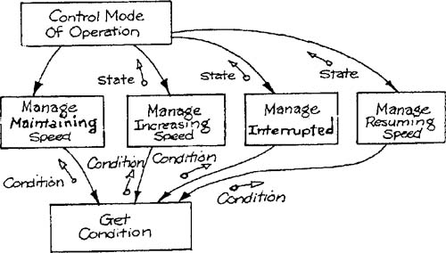
The second strategy for translating a control transformation is to distribute control into several manager modules. This strategy leads to a controlling module that chooses which submodule to call, and one submodule for each state. Each submodule manages all possible transitions from the state, and returns the new state to its caller. A structure chart for the control transformation specification of Figure 9.1 is shown in Figure 9.3.
The code for each of the submodules is to check for conditions that cause a transition, execute the appropriate actions, and return the new state. For example:
module Manage Increase Speed get condition (: condition) if condition = brake then reset Increase Speed flag state ← interrupted else if condition = stop increasing speed then reset increase speed flag record rotation rate set maintain constant speed flag state ← maintaining speed else error ("illegal condition", condition) state ← increasing speed endif endifendmodule
Note that waiting for the condition is placed in the submodule, rather than the controlling module. If a “snapshot” of the task is taken during a test while the task is waiting for a condition, it is possible to know which state the code is in by comparing the address of the suspended task with a load map since, for each state, the task will be waiting for a condition at a different location.
The creation of structure charts from transformation schemas as described in the preceding sections is organized around the logic of a control transformation within the schema. However, it is often necessary to construct all or part of a structure chart from a transformation schema without benefit of a control transformation.
Consider a data transformation that accepts a transaction (that is, a set of data element values) from an operator and uses the information to update stored data; the transformation that changes the equipment configuration for the Defect Inspection System (Appendix D) is of this type. Such a transformation has no inherent control structure; it simply manipulates data and creates outputs when inputs are provided. However, the logic of the transformation may be complex enough to require an implementation with a hierarchy of modules and thus a control structure. This type of transformation may be implemented as a self-contained task, in which case an entire structure chart must be created to represent it. Or it may be within a task controlled by a control transformation, in which case the translation procedure will leave it as a single low-level module to be elaborated into a subhierarchy. The allocation of several isolated transformations to a single task also requires the construction of a hierarchy to control the allocated fragments. In all the above cases, a hierarchy must be built solely from one or more data transformations with no inherent control information.
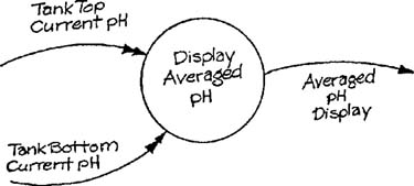
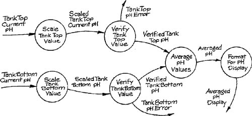
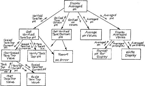
Valuable information for determining the control structure of a structure chart may be gained by decomposing one or more data transformations into a module-level transformation schema. The decomposition process is guided by examining the internal data structure of the original data transformations. This examination can often identify sequential or parallel subtransformations based on required data manipulations. Consider a variation on the Bottle-Filling System transformation (Appendix B in Volume 2) that displays current pH to the area supervisor; assume that the transformation must average two readings from sensors with different characteristics as shown in Figure 9.4. This transformation may receive the sensor readings as arbitrary numeric values, convert them to engineering units, apply reasonableness checks, and convert the average into display format in addition to doing the averaging. The resultant module-level transformation schema is shown in Figure 9.5.
The general categories of intermediate data that may assist in finding subtransformations are:
input data as presented to the task by the environment
input data in essential form
input data in essential form suitable for normal processing
output data in essential form
output data in the form required for export to the environment.
(The decomposition process may aid in the detection of transformation utilities — Figure 9.5 could lead to a general-purpose scaling routine; see the discussion in Section 6.4 of Chapter 6.)
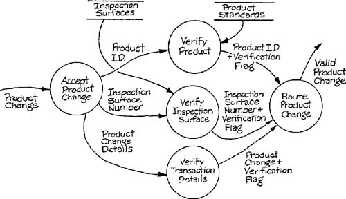
The transformation schema of Figure 9.5 has two parallel streams of transformations because of the separability of the inputs. It is also possible to identify parallelism based on separability of data elements or groups within a single input. Figure 9.6 shows the separation of the components of a transaction that requires verification of identifying data elements against two different data stores.
The module-level transformation schema of Figure 9.5 is the implementation of a single essential model transformation. This type of schema can be translated into a structure chart by a procedure known as transform analysis [1]. The procedure requires identification of the central transform of the schema, which corresponds to the transformation of input in its most essential form into output in its most essential form. There is no exact criterion for identifying a central transform; in practice excluding transformations that validate input, as well as transformations that change data from implementation to essential form or vice versa, leaves one or more transformations that are good candidates for a central transform. The Average pH Values transformation in Figure 9.5 is a reasonable choice. The transformations not belonging to the central transform form one or more streams that are classified as afferent (bearing data to the central transform) and efferent (bearing data away from the central transform). Figure 9.7 shows the schema from Figure 9.5 annotated to show the various regions of the classification.

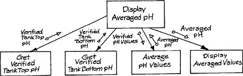
The first stage in the translation consists of creating an upper-level structure chart framework with a controlling module, a second-level module for the central transform, and a second-level module for each afferent and efferent stream (Figure 9.8). All data to and from the afferent and efferent streams is routed through the central transform.
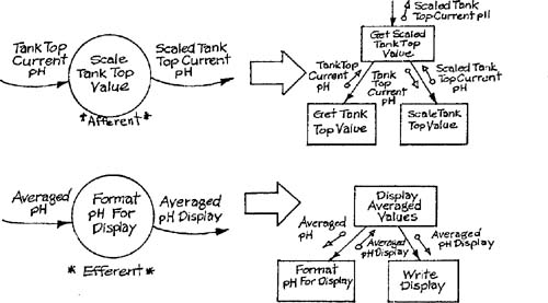
After the framework is established, a subhierarchy is created from each second-level module. If the central transform consisted of a single data transformation, the corresponding module need not be changed; if there were several transformations in the central transform, they can be attached as third-level modules, and all data routed through the upper-level module. The creation of the subhierarchies for the afferent and efferent streams is based on the separation of data movement from data transformation. Although the work of moving data is not explicitly represented on a transformation schema, a single transformation with inputs and outputs implicitly represents the moving of each input to the transformation, the carrying out of the transformation, and the moving of each output from the transformation. Figure 9.9 shows the translation of the components of two transformations into separate modules. The representation differs for afferent and efferent transformations; in the former case the mover of the output is the high-level module, and in the latter case the provider of the input is the high-level module. In both cases, the name of the high-level module reflects the job performed by the entire group of modules.
When a sequence of two or more transformations are to be converted to a structure chart fragment, there are N + l levels in the resulting hierarchy, where N is the number of transformations. For an afferent sequence, the mover of the first transformation’s output merges with the obtainer of the second transformation’s input; for an efferent sequence a similar merging is done. Figure 9.10 shows the structure chart of Figure 9.8 with one afferent and one efferent subhierarchy added; the afferent subhierarchy illustrates the handling of a two-transformation sequence.
If the transformations of the central transform or of the afferent or efferent streams involve decomposition into parallel components as in Figure 9.6, the translation is somewhat different. Figure 9.11 shows the provider of the ultimate output as a top-level module coordinating the obtaining of the input, the processing of the parallel components, and the reconciliation of the results of component processing.
The structure charts produced by transform analysis are referred to as balanced hierarchies. The term means that:
the central transform is isolated from the input and output environments by placement in a separate subhierarchy; and
the highest-level modules are isolated from the low-level details of obtaining data from and sending data to the environment since they see only the net results of low-level module activity.
The transform analysis procedure thus enforces the concept of information hiding, as described in Volume 1, Chapter 4, Modeling Heuristics, and also the separation of essential from implementation details.
The preceding section was restricted to creating the portion of a structure chart corresponding to a single essential model transformation (or the portion of a single transformation assigned to a single task). If several essential model transformations or fragments are assigned to the same task, the structure chart organization must reflect this.
Allocation of several essential transformations to a single task is often necessary because of a time relationship among the essential model pieces (for example, if the required sampling rates are related), or because of task size restrictions. In these cases it is necessary merely to create a module for each essential model fragment, and to subordinate each of these modules to a higher-level coordination module. The high-level module calls the subordinate modules, possibly in an arbitrary order, and enforces any timing relationships such as offsets or activations every other cycle.
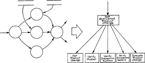
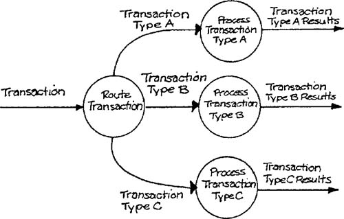
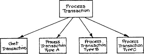
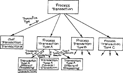
A special case of multiple allocation occurs when several essential model transformations have an input data relationship. Consider the situation illustrated by Figure 9.12, where a transformation accepts an input transaction, checks a “tag,” and distributes the output to the appropriate transformation. This structure is referred to as a transaction center, and the procedure of constructing the structure chart is called transaction analysis [1]. The procedure consists of assigning the identification of type and the routing to a high-level module; modules that obtain the input and that process each type of transaction are called as subordinates, as in Figure 9.13.
Transaction and transform analysis may be combined by using transaction analysis to create the top-level superstructure, then using transform analysis to create a subhierarchy for processing each type of transaction. Figure 9.14 shows one of the subhierarchies added to the structure chart from Figure 9.13. Notice that a shared data area has been used to maintain the movement of data “upward” from the afferent processing to the central transform.
Good design requires that the portion of a system assigned to a task preserve its organization when transformed into code. The structure chart, which describes the code organization, must thus be created so as not to distort the organization of the transformation schema. The translation techniques introduced in this chapter have as a goal the preservation of this organization.