The WHERE clause is all about true conditions. Its basic syntax is:

WHERE condition that evaluates as TRUE

As we’ve learned, a condition is some expression that can be evaluated by the database system. The result of the evaluation will be one of TRUE, FALSE, or UNKNOWN. We’ll cover these one at a time, starting with TRUE.

SELECT
  name
FROM
  teams
WHERE
  id = 9

WHERE condition that evaluates as TRUE 

WHERE ( NOT id ) = 9

WHERE NOT ( id = 9 ) 

WHERE id <> 9 

WHERE id != 42 

So far, we’ve seen the Teams application, briefly, in Chapter 1, and the Content Management System application, in more detail, in Chapter 2 and Chapter 3.

Our next sample application, Shopping Carts, supports an online store for a web site, where site visitors can select items from an inventory and place them into shopping carts when ordering. Anyone who’s ever made a purchase on the Web will already be familiar with the general features of online shopping carts. In case you’re thinking that shopping carts are complex—and they are—our Shopping Carts sample application is very simple in comparison to a real one. It’s not meant to be industrial strength; it’s just a sample application, intended to allow us to learn SQL.

The first table we’ll look at in the Shopping Carts application is the items table. This table will contain all the items that we plan to make available for purchase online. Figure 4.1 shows the items table after its initial load of data.

Figure 4.1. The items table

Notice that some of the prices are empty in the diagram. These empty values are actually NULL. I haven’t discussed NULL in detail yet, although we met NULL briefly in Chapter 3: NULLs were returned by outer joins in the columns of unmatched rows.

What does it mean that the price of certain items is NULL? Simply that the price for that item is not known—yet. Obviously, we can’t sell an item with an unknown price, so we’ll have to supply a price value for these items eventually. NULL can have several interpretations, including unknown and not applicable. In the case of outer joins, NULLs in columns of unmatched rows are best understood as missing. In the items table example, the price column is NULL for items to which we’ve not yet been assigned a price, so the best interpretation is unknown.

How does all this talk about NULL relate to conditions in the WHERE clause? Let’s look at a sample query:

SELECT
  name
, type
FROM
  items
WHERE
  price = 9.37

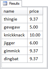
Here the WHERE clause consists of just one condition: the value of the price column must be 9.37 for that row to be returned in the result set. And the result set, shown in Figure 4.2, produced by this query is exactly what we’d expect.

Figure 4.2. Using a simple WHERE clause

As we learned earlier, the condition in the WHERE clause is evaluated on each row, and only those rows where the condition evaluates as TRUE are retained. So what happens when the WHERE clause is evaluated for items that have NULL in the price column? For these rows, the evaluation is UNKNOWN.

WHERE clause conditions can utilize many other operators besides equal and not equal. These other operators are mostly straightforward and work just as we would expect them to.

SELECT
  name
, type
FROM
  items
WHERE
  price < 10.00

WHERE name < 'C'

WHERE created >= '2009-04-03'

The LIKE Operator

The LIKE operator implements pattern matching in SQL: it allows you to search for a pattern in a string (usually in a column defined as a string column), in which portions of the string value are represented by wildcard characters. These are a small set of symbolic characters representing one or more missing characters.

For example, consider the query:

Cart_02_LIKE_and_BETWEEN.sql (excerpt)

SELECT
  name
, type
FROM
  items
WHERE
  name LIKE 'thing%'

The results of this query are shown in Figure 4.3.

In standard SQL, LIKE has two wildcards: the percent sign (%), which stands for zero or more characters, and the underscore (_), which stands for exactly one character. Notice how in the query above, name values which satisfied the WHERE condition each start with the characters thing, followed by zero or more additional characters. Thus, these values match the pattern specified by the LIKE string, so the condition evaluates as TRUE.

Figure 4.3. Using a wildcard in a query

The BETWEEN Operator

The purpose of the BETWEEN operator is to enable a range test to see whether or not a value is between two other values in its sequence of comparison. A typical example is:

Cart_02_LIKE_and_BETWEEN.sql (excerpt)

SELECT
  name
, price
FROM
  items
WHERE
  price BETWEEN 5.00 AND 10.00

The way BETWEEN works here is fairly obvious. Items are included in the result set if their price is between 5.00 and 10.00, as the result set in Figure 4.4 shows.

Figure 4.4. Using a BETWEEN operator

The BETWEEN range test is actually equivalent to the following compound condition, in which two conditions—in this case 5.00 <= price and price <= 10.00—are combined:

WHERE
  5.00 <= price AND price <= 10.00

There are two important aspects to note here.

• The first is the sequence. 5.00 has to be less than or equal to price, and price has to be less than or equal to 10.00. In other words, the smaller value comes first, and the larger value comes last, with the value being tested coming between them. If the actual value does not lie between the endpoints, the BETWEEN condition evaluates as FALSE.

• The second important detail to notice is that the endpoints are included.

BETWEEN: It haz a flavr

Here are two examples which will illustrate the flavor or correct usage of BETWEEN.^[3] In the first example, we want to return all entries posted in the last five days:

WHERE
  created BETWEEN CURRENT_DATE AND CURRENT_DATE - INTERVAL 5 DAY

Here, CURRENT_DATE is a special SQL keyword that always corresponds to the current date when the query is run. Furthermore, the CURRENT_DATE - INTERVAL 5 DAY expression is the standard SQL way of doing date arithmetic (because that’s a minus sign rather than a hyphen). Yet this WHERE clause fails to return any rows at all, even though we know that there are rows in the table with a created value within the last five days. What’s going on?

Let’s assume that the CURRENT_DATE is 2009-03-20, which would mean that CURRENT_DATE - INTERVAL 5 DAY is 2009-03-15. The WHERE clause is then equivalent to:

WHERE
  created BETWEEN '2009-03-20' AND '2009-03-15'

This might look okay, but it isn’t. Syntactically, it’s fine, but semantically, it’s flawed. The flaw can be seen more easily if we rewrite the BETWEEN condition using the equivalent compound condition:

WHERE
  '2009-03-20' <= created AND created <= '2009-03-15'

Now, there may be some rows with a created value that is greater than or equal to 2009-03-20. There may also be some rows with a created value that is less than or equal to 2009-03-15. However, the same created value, on any given row, cannot simultaneously satisfy both conditions. Our mistake is to have placed the larger value first. Remember, with dates, smaller means chronologically earlier. The original WHERE clause should have been written with the earlier date first, like this:

WHERE
  created BETWEEN CURRENT_DATE - INTERVAL 5 DAY AND CURRENT_DATE

Our second example of correct BETWEEN usage concerns the endpoints. Consider the following WHERE clause, intended to return all entries for February 2009:

WHERE
  created BETWEEN '2009-02-01' AND '2009-03-01'

This is fine, except that it includes entries posted on the first of March, which is outside the date range we’re aiming for. Immediately, you might think to rewrite this as follows:

WHERE
  created BETWEEN '2009-02-01' AND '2009-02-28'

This is correct, but inflexible. If we wanted to generalize this so that it returns rows for any given month, we would need to calculate the last day of the month; this can become extremely hairy, as anyone can attest who’s coded a general date expression that takes February 29 into consideration. The best-practice approach in these cases, then, is to abandon the BETWEEN construction and code an open-ended upper endpoint compound condition:

WHERE
  '2009-02-01' <= dateposted AND dateposted < '2009-03-01'

Notice that the second comparison operator is solely less than, not less than or equal. All values of created greater than or equal to 2009-02-01 and up to, but not including, 2009-03-01, are returned.

The compound condition is usually written like this, for convenience:

WHERE
  created >= '2009-02-01' AND created < '2009-03-01'

The only requirement then is to calculate the date of the first day of the following month, rather than try to figure out when the last day of the month in question is.

Compound conditions—multiple conditions that are joined together—in the WHERE clause are common. Here’s an example:

SELECT
  id
, name
, billaddr
FROM
  customers
WHERE
  name = 'A. Jones' OR 'B. Smith'

It’s clear what is meant here—return all rows from the customers table that have a name value of 'A.Jones' or 'B.Smith'. Unfortunately, this produces a syntax error, because 'B.Smith', by itself, is not a condition except in MySQL. In MySQL the string is interpreted by itself as FALSE, so the compound condition above is equivalent to “name equals 'A.Jones' (which may or may not be true), or FALSE.”

The correct way to write the compound condition shown above would be:

WHERE
  name = 'A.Jones' OR name = 'B.Smith'

WHERE 
  customers.name = 'A.Jones' OR customers.name = 'B.Smith'
      AND items.name = 'thingum'

WHERE 
  customers.name = 'A.Jones'
      OR ( customers.name = 'B.Smith' AND items.name = 'thingum' )

WHERE 
  ( customers.name = 'A.Jones' OR customers.name = 'B.Smith' )
      AND items.name = 'thingum'

WHERE
  1=1  
      AND type = 'widgets'
      AND price BETWEEN 10.00 AND 20.00

WHERE
  1=0
      OR name LIKE '%Toledo%'
      OR billaddr LIKE '%Toledo%'
      OR shipaddr LIKE '%Toledo%'

You’ll recall this example from the section on AND and OR:

WHERE 
  ( customers.name = 'A.Jones' OR customers.name = 'B.Smith' )
      AND items.name = 'thingum' 

There’s another way to write this:

WHERE 
  customers.name IN ( 'A.Jones' , 'B.Smith' )
      AND items.name = 'thingum'

In this version, we’ve moved the parentheses to be part of the IN condition rather than being used to control the evaluation priority of AND and OR. The IN condition syntax consists of an expression, followed by the keyword IN, followed by a list of values in parentheses. If any of the values in the list is equal to the expression, then the IN condition evaluates as TRUE. Should you wish to set the condition to check if a value is not in a list of values, you can prefix the IN condition with the NOT keyword:

WHERE
  NOT ( customers.name IN ( 'A.Jones', 'B.Smith' ) )

You could also write this as:

WHERE
  customers.name NOT IN ('A.Jones', 'B.Smith')

Note that while the NOT keyword can be used with an IN condition in these two ways, this doesn’t always apply to other operators. For example, it’s perfectly okay to write:

WHERE
  NOT ( customers.name = 'A.Jones' )

However, it’s not okay to write:

WHERE
  customers.name NOT = 'A.Jones' 

Another reason I prefer to place NOT in front of a parenthesized condition is that it’s easier to spot it in a busy WHERE clause (that is, one which has many conditions) than a NOT keyword buried inside a condition.

SELECT
  name
FROM
  items
WHERE 
  id IN (
    SELECT
      cartitems.item_id            
    FROM
      carts          
        INNER JOIN cartitems
          ON cartitems.cart_id = carts.id           
    WHERE
      carts.customer_id = 750
  )

Since this chapter is all about the WHERE clause, this is the appropriate context in which to discuss the concept of correlation. In this context, a subquery correlates (co-relates) to its parent query if the subquery refers to—and is therefore dependent on—the parent to be valid.

A correlated subquery can’t be run by itself, because it makes reference—via a correlation variable— to the outer or main query. To demonstrate, let’s work through an example based on the entries table in the Content Management System application that we saw in Chapter 3. This is shown in Figure 4.5.

Figure 4.5. The CMS entries table

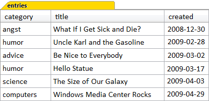
The example will use this table in the outer query, and have a correlated subquery that obtains the latest entry in each category based on the created date:

SELECT
  category
, title
, created
FROM
  entries AS t
WHERE
  created = (
    SELECT
      MAX(created)
    FROM
      entries
    WHERE
      category = t.category
  )

Let’s start looking at this by reviewing the subquery first. There are two features to note here:

In essence, what this query does can be paraphrased as: “return the category, title, and created date of all entries, but only if the created date for the entry being returned is the latest created date for all the entries in that particular category.” Or, in brief, return the most recent entry in each category. The correlation ensures that the particular category is taken into consideration to determine the latest date, which is then used to compare to the date on each entry, as shown in Figure 4.6.

Figure 4.6. How correlation works

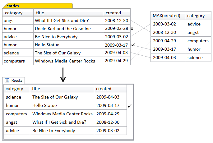
In this example, a comparison is made between each entry’s created value, and the maximum created value of all rows in that category, as produced by the subquery. If that entry contains the same date for its category as found by the subquery, it’s returned in the result set. If it’s not the same date, it’s discarded.

Because this is a very simple example, only one category actually has more than one entry: humor. The subquery determines that “Hello Statue” has the most recently created date, and thus discards "Uncle Karl and the Gasoline."

If Figure 4.6 reminds you of Figure 3.11 (which demonstrated how an inner join worked), remember that the distinguishing characteristic of a correlated subquery is that it’s tied to an object in the outer or main query, and can’t be run on its own. Joins, on the other hand, are part of the main query.

Aside from that, the inner join and the correlated subquery are quite similar. In the join, the rows of the categories and entries tables were joined, based on the comparison of their category columns in the join condition. In the correlated subquery, the rows of the entries table are compared to the rows of the tabular result set produced by the correlated subquery, and if this somehow reminds you of a join, full marks. In fact, correlated subqueries can usually be rewritten as joins.

Here’s the equivalent query written using a join instead of a correlated subquery:

SELECT
  t.category
, t.title
, t.created
FROM
  entries AS t
    INNER JOIN (
      SELECT
        category
      , MAX(created) AS maxdate
      FROM
        entries 
      GROUP BY
        category
    ) AS m
      ON m.category = t.category AND m.maxdate = t.created

The join version employs a subquery as a derived table, containing a GROUP BY clause. We’ll cover the GROUP BY clause in detail in Chapter 5, but for now, please just note that the purpose of the GROUP BY here is to produce one row per category. So the subquery produces a tabular result set consisting of one row per category, and each row will have that category’s latest date, which is given the column alias maxdate. Then the derived table, called m, is joined to the entries table, which uses the table alias t. Notice that there are two join conditions. You can see both of these conditions in the correlated subquery version, too—one inside the subquery (the category correlation), and the other in the WHERE clause (where maxdate in the subquery should equal the created date in the outer query).

An EXISTS condition is very similar to an IN condition with a subquery. The difference is that the EXISTS condition’s subquery merely needs to return any rows, be it a million or just one, in order for the EXISTS condition to evaluate to TRUE. Furthermore, it does not matter what columns make up those rows—merely that some rows exist (hence the name).

To demonstrate the use of EXISTS, we’ll use the Shopping Cart sample application again, but this time focus on the customers and their carts. To put these terms in context here, a customer is a person who has registered on the web site, and a cart is the collection of items that the customer has selected for purchase. Let’s say we want to find all the customers who have yet to create a cart. The key idea here is the not part of the requirement, so we’ll use NOT EXISTS in the solution:

SELECT
  name
FROM
  customers
WHERE
  NOT EXISTS (
    SELECT
      1 
    FROM
      carts
    WHERE
      carts.customer_id = customers.id
  )

As you can see, we're using a correlated subquery again within the WHERE clause. This time, the correlation variable is not a table alias, but rather just the name of the table in the outer query. In other words, the subquery will return rows from the carts table where the cart’s customer_id column is the same as the id column in the customers table in the outer or main query. If a customer has one or more carts, as returned by the subquery, EXISTS would evaluate to TRUE. However, we're using NOT EXISTS in the main query so a customer's name will only be included in the result set if there are no carts for the customer returned by the subquery, exactly as required.

But what, you may well ask, is SELECT 1 all about? Well, as noted earlier, the EXISTS condition does not care which columns are selected, so SELECT 1 simply returns a column containing the numeric constant 1. The subquery could just as easily have selected the customer_id column. EXISTS will evaluate TRUE or FALSE, no matter which columns the subquery selects. We’ll cover the SELECT clause in detail in Chapter 7.

SELECT
  name
FROM
  customers
WHERE
  NOT (
    id IN (
      SELECT
        customer_id
      FROM
        carts
    )
  )

SELECT
  name
FROM
  customers AS t
WHERE
  NOT (
    id IN (
      SELECT
        customer_id
      FROM
        carts 
      WHERE 
        customer_id = t.customer_id
    )
  )

SELECT
  customers.name
FROM
  customers
    LEFT OUTER JOIN carts
      ON customers.id = carts.customer_id
WHERE 
  carts.customer_id IS NULL

We’ve just seen four different ways to write an SQL query to achieve a specific result:

In practice, which of these is the best approach to take? Generally, you should let the database system optimize your queries for performance. The database optimizer—the part of the database system which parses our SQL, and then figures out how to obtain the data as efficiently as possible—is a lot smarter than many people think. It may realize that it doesn’t have to retrieve any carts at all!

Let’s consider what the LEFT OUTER JOIN version of the previous example is doing. The query will retrieve all carts for all customers, including customers who have no cart (since it’s a LEFT OUTER JOIN); then the WHERE clause throws away all rows retrieved, except those rows for customers who have no cart. Seems wasteful, doesn’t it? And it might well be … if it were an accurate portrayal. It’s unnecessary to actually retrieve any cart rows; what’s needed is simply to know which customers don’t have one. So the left outer join with an IS NULL test is the same, semantically, as the NOT EXISTS version.

What about the correlated and uncorrelated subqueries using the NOT IN condition? How will they perform? Here’s one way to think about what they’re doing: the uncorrelated subquery retrieves a list of customer_ids from all carts, and then, in the outer query, checks each customer’s id against this list, keeping those customers whose id is not in the list. The correlated subquery retrieves the customer_id from individual cart rows, but only the cart rows for that customer. Yet in the end, the correlated query will actually have retrieved all the cart rows too (like the uncorrelated query did), even though it keeps only those customers who don’t have a cart, as well. So it would seem that these queries, too, might wastefully retrieve all carts.

Intuition alone cannot lead us to a happy conclusion here. Our next step might be to test all versions and see how they fare. More often than not, they will all perform the same; ultimately, we’ll need to base our analysis on some facts, and for that, we need to do some research. See the section called “Performance Problems and Obtaining Help” in Appendix A for some ideas on how to proceed.

We covered a lot of ground in this chapter, but the main points that you should take away from it are:

In Chapter 5, we'll look at the GROUP BY clause, which operates on the rows produced by the FROM clause that weren’t filtered out by the WHERE clause.