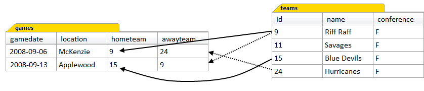
Figure 11.1 depicts a portion of the data model diagram for the Teams and Games application, where the teams table is related to the games table twice. Why would we want to do this? The answer: each game involves two different teams. In every game, one of the teams is the home team, and another team is the away team. Thus, two relationships are needed.

Figure 11.1. The teams table is related to the games table twice

Using the diagramming convention introduced in Chapter 10, the arrows indicates the cardinality of the one-to-many relationship. This data model shows that:

Following the arrows in the data model diagram from the games entity to the teams entity—in the many-to-one direction—we can see that each game can have only one home team, and one away team. The details of the relationship are unspecified in the diagram in Figure 11.1, with no mention of home and away teams; obviously you would annotate the diagram properly, though, if you produce diagrams for your own use or in a professional team environment.

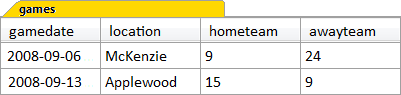
Figure 11.2 shows the data in the games table. The first detail you may notice is that the hometeam and awayteam columns are numbers, not names. These columns are foreign keys that correspond to values of the primary key id column in the teams table. The SQL for the creation of the games table can be found in the section called “The games Table” in Appendix C.

Figure 11.2. The games table

So the design of this special structure is fairly straightforward, but to produce a report or display that’s useful, we’ll need to use team names instead of the foreign key values. We’ll need to perform two lookups, to translate the foreign keys into names. The SQL that’s needed to display team names seems to give many developers trouble.

This is where joining to a table twice comes in. To retrieve the team names, we need to join the games table to the teams table, but we need to use both of the foreign key columns. This, in turn, requires that we use two joins:

SELECT
  games.gamedate
, games.location
, home.name AS hometeam
, away.name AS awayteam
FROM
  games
    INNER JOIN teams AS home 
      ON home.id = games.hometeam
    INNER JOIN teams AS away 
      ON away.id = games.awayteam

Each of the inner joins in this query joins the same row of the games table to a different row of the teams table—one being the home team, and the other being the away team. Figure 11.3 illustrates what’s happening in the joins.

Figure 11.3. The teams table joined to the games table twice

The result of the query is shown in Figure 11.4. In short, we’ve joined the games table to the teams table twice, and thereby enabled two separate queries. The important point to note here, is that we need to use table aliases to accomplish this. In any query that references two representations of the same table, we must always use table aliases to distinguish them.

Figure 11.4. Team names in the result set

In addition, the query uses column aliases on two of the columns in the SELECT clause. (The column aliases hometeam and awayteam are actually the same names as the foreign key columns in the games table. This is a mere coincidence; any two different names will serve.) The purpose of the column aliases is to distinguish the home team from the away team. Without the column aliases, the result set would have two columns called name.

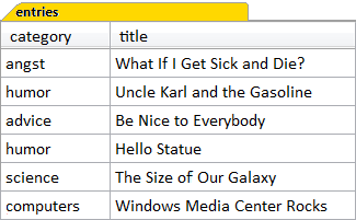
We saw categories and entries in some detail in Chapter 3, in which the relationship between categories and entries was examined in the context of the various types of joins. Figure 11.5 shows the entries table, where the category column is a foreign key to the category column of the categories table, which is its primary key. This is, of course, not the whole entries table—it’s missing some columns—just a simplified version for our purposes here. The categories table is shown in Figure 11.6.

Figure 11.5. The entries table

Figure 11.6. The categories table

Now let’s say that we want to distinguish further between our categories of entries. We have a curious mix of different kinds of entries here—some are objective, analytical, and factual, whereas others are subjective, personal, and pensive. What we want to do is set up two new super-categories, General and Personal, as shown in Figure 11.7. This classification of our original categories into General and Personal would allow us, for example, to display entries from these categories using different themes.

Figure 11.7. The new super-categories

Other than calling them super-categories, we can call them categories and demote the old categories to subcategories. The category/subcategory structure is implemented with a foreign key from the categories table to itself. Figure 11.8 shows the actual data once this relationship has been created. You can have a look at the SQL query that achieves this in the section called “The categories Table” in Appendix C. Notice that the new column, parent, contains values which are the same values as used in the category column—except in the first two rows. A category is determined to be a subcategory when it has a parent category value.

Figure 11.8. The categories table with the new parent column

Figure 11.9 shows a portion of the data model diagram for the Content Management System application representing the relationship between categories and entries.

Figure 11.9. The relationship between categories and entries

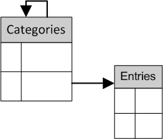
You may be wondering about that funny-looking relationship from the categories table to itself. This is a reflexive relationship (sometimes called a recursive relationship). It’s a one-to-many relationship because each category can have multiple subcategories, but each subcategory can have only one (parent) category.

Finally, we’re ready to see an example of a query that joins a table to itself. We’ll start with a query to list our categories and subcategories alphabetically:

SELECT
  cat.name AS supercategory
, sub.name AS category
FROM
  categories AS cat
    INNER JOIN categories AS sub 
      ON sub.parent = cat.name
ORDER BY 
  cat.name
, sub.name

The results of this query are shown in Figure 11.10.

Figure 11.10. Results of the categories table joined to itself

So the categories table is being self-joined, or joined to itself, using a join condition which matches the foreign key of one row to the primary key of another row in the same table. The ON clause specifies that the sub row’s parent column value must match the cat row’s category column value. Figure 11.11 illustrates what’s occurring in the join.

Figure 11.11. The categories table is being joined to itself

The lines in the diagram above indicate the only pairs of cat and sub rows that actually match. It’s an inner join, and since NULL equals no value, two of the sub rows are unmatched with any cat row. This is because the General and Personal categories do not themselves have parent categories.

Using categories and subcategories in a database is a common requirement. For instance, we often see them in a web site’s navigation bar or site map. Our application’s programming language helps us easily transform the result set in Figure 11.10 to the following HTML:

<ul>
  <li>Articles and Resources
    <ul>
      <li>Information Technology</li>
      <li>Our Spectacular Universe</li>
    </ul>
  </li>
  <li>Personal Stories and Ideas
    <ul>
      <li>Gentle Words of Advice</li>
      <li>Humourous Anecdotes</li>
      <li>Log On to my Blog</li>
      <li>Stories from the Id</li>
    </ul>
  </li>
</ul>

The transformation logic is a bit beyond the scope of this book, but involves looping over the rows of the result set and detecting control breaks in the super-category name—a technique introduced in the section called “ASC and DESC” in Chapter 8.

Finally, let’s take our query one step further, and join the categories to the entries table as well:

SELECT
  cat.name AS supercategory
, sub.name AS category
, entries.title
FROM
  categories AS cat
    INNER JOIN categories AS sub 
      ON sub.parent = cat.category
    LEFT OUTER JOIN entries 
      ON entries.category = sub.category
ORDER BY
  cat.name
, sub.name
, entries.title

Using a left outer join, we join the entries table to the result set of joining the categories table to itself. The result, shown in Figure 11.12, is a result set listing all entries with three columns: supercategory, category, and title. Because we used a left outer join to join to the entries table, we have a NULL in the title column for the Log on to My Blog category.

Figure 11.12. Super-categories, categories, and titles

Keywords are a very common feature of many different types of applications; you may see them implemented as tags in web applications where users tag entries with topic-related keywords. In our Content Management System application, entries may have one or more keywords, and the same keyword may be applied to multiple entries. So the relationship between entries and keywords is a many-to-many relationship. This relationship is shown in Figure 11.13.

Figure 11.13. The relationship between entries and keywords in the CMS

However, when we’re in the implementation stage of our data model, that is, when we’re creating tables for the entities defined by our model, each many-to-many relationship must be broken down into two, one-to-many, foreign-key relationships. Knowing this, most data modellers simply introduce a relationship entity into the model. In this case, the relationship between entries and keywords is implemented via two one-to-many relationships, with the EntryKeywords entity—on the arrowhead end of both relationships in our ER diagram in Figure 11.13.

Lets first examine the data in our sample CMS application. Figure 11.14 shows the id (the primary key) and title columns from the entries table.

Figure 11.14. The entries table

Figure 11.15 shows the new entrykeywords table, where entry_id is a foreign key, referencing the id of the entries table, so this is just another typical one-to-many relationship. The SQL for the creation of this table can be found in the section called “The entrykeywords Table” in Appendix C.

Figure 11.15. The entrykeywords table

The primary key of the entrykeywords table is a composite key consisting of both columns, since we only want a keyword to be assigned to an article once. Any query which needs to return entries along with their keywords will have to perform a join between the entries and the entrykeywords tables, using the primary key and foreign key relationship depicted in Figure 11.16.

Figure 11.16. A join between the entries and entrykeywords table

In most situations, to achieve this result, a left outer join from entries to entrykeywords is used. You might like to use an inner join, however, if you’re interested only in entries that have had at least one keyword assigned.

At this point, it would seem that our many-to-many relationship has been successfully implemented using only two tables, so why do we need a third? As it’s implemented at the moment, we can insert rows into the entrykeywords table using whatever keywords we like; the keyword column in the entrykeywords is simply a data column, as opposed to a foreign key column. (It should still be a part of the primary key, though, so that we avoid inserting the same keyword more than once for each entry.)

This is another one of those delightful instances where the choice is up to you. As it stands any keywords can be inserted into the entrykeywords table. However, if your application should only allow a restricted set of keywords to be used, then you’ll need to implement the second one-to-many relationship and make a third table for keywords.

This new keywords table will contain the list of keywords that can be associated with entries. Using a foreign key constraint, we can make sure that only keywords that are in the keywords table can be added to an entry. Of course, this will also mean that if a new keyword is introduced, it will have to be added to the keywords table first before it can be added to an entry.

We could implement the keywords table with two columns: an id column for the primary key (possibly a surrogate key, like an autonumber) and a keyword column for the keyword itself. The entrykeywords table should then be modified so that the keyword column becomes a foreign key column; that way it references the values from the id column in the new keywords table.

With an implementation like that, any query which needs to return entries along with their keywords will have to perform a join between the entries and the entrykeywords tables, and then between the entrykeywords table and keywords table, using the primary key and foreign key relationship. To me, this hardly seems worth the effort!

If all we’re doing is ensuring that only the keywords in the keywords table are used for entries, it really only needs one column—the keyword column—as it’s a perfect natural key; the surrogate primary key column is entirely redundant in this situation. Figure 11.17 illustrates the relationship between entrykeywords and a one-column keywords table.

Figure 11.17. The relationship between entrykeywords and keywords

With the keywords table in place (and the foreign key relationship defined between the entrykeywords table to the keywords table), we simply add a new keyword to the keywords table, and then we can start assigning it to entries. We’ll only be able to assign a new keyword to an entry if that keyword has been inserted beforehand in the keywords table. Since we’re using a natural key (the keyword itself) instead of a surrogate key, we know that every foreign key value must have a matching primary key value. There’s no need to perform a join operation to retrieve them, because they’re going to be the same as the keyword values in the entrykeywords table.

Tip: The MySQL Function GROUP_CONCAT

MySQL has a wonderful aggregate function called GROUP_CONCAT. In a nutshell, it works on strings the same way that SUM works on numbers. The GROUP_CONCAT function concatenates the values in a character column, using an optional separator—the default being a comma.

This function is supremely useful in many situations where data from multiple relationships must be retrieved. It allows one of those relationships to be collapsed to one row per entity. Here’s an example using entries and keywords:

(excerpt)

SELECT
  entries.title
, GROUP_CONCAT(entrykeywords.keyword) AS keywords
FROM
  entries
    LEFT OUTER JOIN entrykeywords
      ON entrykeywords.entry_id = entries.id
GROUP BY
  entries.title

The results of this query are shown in Figure 11.18. All of the keywords for each entry_id have been concatenated into a single value (but separated by commas within the single value), and placed in the row for the matching entry id value.

Figure 11.18. The results using GROUP_CONCAT

We started with a many-to-many relationship in the original data model, but ended up implementing only half of the two one-to-many table relationships needed to support it. This is actually very common; the one half of a many-to-many structure is used for numerous other applications besides keywords and tags. As you work with databases, keep an eye open. Whenever you encounter a one-to-many relationship between two tables, ask yourself whether there needs to be another table—to complete the other half of a many-to-many relationship—and if a surrogate key is really necessary.

In this chapter, we learned about three types of special structures that occur often in applications:

This concludes the chapters on database design, and also the book.

Don’t forget that there’s a web site that goes along with this book, located at http://www.sitepoint.com/books/sql1/, where you can also obtain the actual SQL script files used we’ve used.

There’s a lot more to SQL than what we’ve covered in this book. SQL is like chess—you can learn the basics in a couple of hours, but it takes a long time to become a grand master. There is, however, only one way to become better: practice, practice, practice!