Grouping is more than simply sequencing data. Sequencing simply means sorting the data into a certain order. Grouping does involve an aspect of sequencing, but it goes beyond that. To demonstrate, we'll first review the data in our sample Shopping Cart application tables, and then work through several GROUP BY queries to see how grouping affects the results.

Our first goal, therefore, is to write a query that produces a result set that displays a useful set of data from our application, much like the queries we’ve been writing so far. To make the distinction between the queries we’ve used up till now and a query involving grouping, we call this type of query a detail query because it returns detail rows—the columns and rows of data as they are stored in the database tables—ungrouped. The distinction between detail rows and group rows is important and will become clear shortly.

As always, the first item to write is the FROM clause. The sample Shopping Cart application data is spread out over several tables, so we’ll need to bring it together with a join query:

FROM
  customers 
    INNER JOIN carts
      ON carts.customer_id = customers.id
    INNER JOIN cartitems
      ON cartitems.cart_id = carts.id 
    INNER JOIN items
      ON items.id = cartitems.item_id

This query joins four tables together. We haven’t seen a quadruple join before, so we’ll walk through it slowly and examine each join in turn. It may help to look back at the FROM clause as we walk through the joins.

The FROM clause starts with the customers table. Then the carts table is joined to the customers table, based on the customer_id in each row of the carts table matching the corresponding id in the customers table. We’re on solid ground here, because all our previous join examples have involved two tables.

Then the cartitems table is joined, based on the cart_id in each row of the cartitems table matching the corresponding id in the carts table. This is now the third table in the join, and it might help to think of this third table as being joined to the tabular structure produced by the join of the first two tables. Since that tabular structure consists of the matched rows of the first two tables joined or concatenated together (to form a wider tabular structure), the join of the third table is, in effect, a join of two tabular structures again: the tabular structure produced by joining the first two tables, to which the third table is joined. You’re probably ahead of me here, but I still need to say it: the result of joining the third table is yet another tabular structure.

Finally, the items table is joined, based on the id in the items table matching the corresponding item_id in the cartitems table. This is the fourth table, and it joins the tabular structure produced by the join of the previous three.

SELECT
  *
FROM …

Retrieving the entire tabular result set produced by the four table join is too much detail for our purposes here. There are many extraneous columns that would be in the way of trying to understand the available data, as we prepare to use our first GROUP BY clause. Therefore, we’ll specify only a few carefully chosen columns in the SELECT clause:

SELECT
  customers.name    AS customer
, carts.id          AS cart
, items.name        AS item
, cartitems.qty
, items.price
, cartitems.qty
      * items.price AS total
FROM
  …

We’ve yet to cover the SELECT clause in detail (we will in Chapter 7), but we’ve certainly seen it before; in this particular case, the columns are straightforward, with perhaps the exception of the last line. This expression computes the total price of each item in a cart by multiplying its price by the amount of that item in the cart.

We’ll also add an ORDER BY clause:

  …
ORDER BY 
  customers.name
, carts.id
, items.name

The purpose of the ORDER BY clause here is to sort the result set into the specified sequence: first by customer name, then the cart ID, and then the item name. We’ll examine this clause in detail in Chapter 8.

Our completed detail query looks like so:

SELECT 
  customers.name    AS customer
, carts.id          AS cart
, items.name        AS item
, cartitems.qty
, items.price
, cartitems.qty 
      * items.price AS total
FROM
  customers
    INNER JOIN carts 
      ON carts.customer_id = customers.id
    INNER JOIN cartitems 
      ON cartitems.cart_id = carts.id 
    INNER JOIN items 
      ON items.id = cartitems.item_id
ORDER BY
  customers.name
, carts.id
, items.name

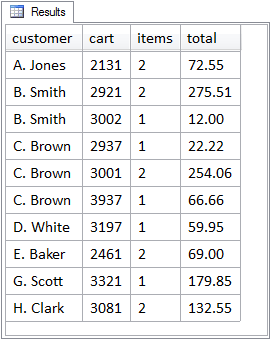
Figure 5.1 shows the result set the detail query produces: several customers, the carts that they created, and the items in those carts, together with the quantity of the items purchased, the price of each item, and the total price for that quantity.

Figure 5.1. The results of the detail query: all the customers, carts, and items

Notice that the customers are in sequence. Within each customer, the carts are in sequence (if there is more than one per customer), and within each cart, the items are in sequence by name. This sequencing was accomplished by the ORDER BY clause, which was used so we could see the customers-to-carts and carts-to-cartitems relationships in the data more easily (they would be harder to spot if the rows came back in random order, for example).

So to recap what we’ve seen in the results for the detail query:

You may well be wondering at this point, “Yes, that’s nice, it makes sense, and I can see the query results are sorted nicely, but what has this to do with GROUP BY?” The reason for looking at the detail data carefully, and in this particular sequence, is to see how the items for a cart are grouped together, and how the carts for a customer are grouped together. However, this is not the grouping that the GROUP BY clause produces; it is merely the sequencing that the ORDER BY clause produces. In other words, if we want to see detailed row data “grouped” into a certain sequence, we use ORDER BY. GROUP BY has another purpose altogether.

The role of the GROUP BY clause is to aggregate, meaning to collect together, or unite. Let’s look at our first example of a query that uses a GROUP BY clause:

SELECT 
  customers.name      AS customer
, carts.id            AS cart
, COUNT(items.name)   AS items
, SUM(cartitems.qty
      * items.price)  AS total
FROM 
  customers 
    INNER JOIN carts 
      ON carts.customer_id = customers.id
    INNER JOIN cartitems 
      ON cartitems.cart_id = carts.id 
    INNER JOIN items 
      ON items.id = cartitems.item_id
GROUP BY 
  customers.name
, carts.id

This is almost the same as the detail query; it has the same FROM clause, but there are some slight differences in the SELECT clause, and the GROUP BY clause is new.

The SELECT clause now contains two common aggregate functions, COUNT and SUM. As you might have guessed, COUNT counts rows, and SUM produces a total. We'll look at these and other aggregate functions in more detail in Chapter 7.

The GROUP BY clause contains the names of two columns: customers.name and carts.id. In doing so, the GROUP BY clause will produce one row, a group row or aggregate row, in the query's result set for every distinct combination of the values in the columns specified. The tabular structure shown in Figure 5.2 is the result set returned by the above query. Instead of detail rows, we now have group rows.

Figure 5.2. Results of the GROUP BY query

The items column in this result set is the number of items in each particular cart, while the total column is the sum of the individual line item totals on the cart. Where a customer cart includes more than one item, those multiple item rows have been aggregated into one row per cart per customer. There are still multiple rows per customer, but there is now only one row per cart per customer.

The GROUP BY clause has aggregated the rows for each customer cart, producing one out of many, while the COUNT and SUM functions have computed the aggregate quantities—a count and a sum—for all those rows taken together. Hence, the presence of the GROUP BY clause has created group rows from the detail rows of the tabular result set, which was produced from the FROM clause.

Figure 5.3 illustrates the grouping concept by showing the results of the detail query and the results of the above GROUP BY query, side by side. Note that the grouping columns have been highlighted, and some spacing has been inserted, to make it easier to see the grouping.

Figure 5.3. Comparing detail rows to group rows—two column grouping

Let’s write another example using the GROUP BY clause:

SELECT 
  customers.name      AS customer
, COUNT(items.name)   AS items
, SUM(cartitems.qty 
      * items.price)  AS total
FROM 
  customers 
    INNER JOIN carts
      ON carts.customer_id = customers.id
    INNER JOIN cartitems
      ON cartitems.cart_id = carts.id 
    INNER JOIN items
      ON items.id = cartitems.item_id
GROUP BY 
  customers.name

This is practically the same query as before, except that in this case, the GROUP BY clause contains only one column, customers.name. Thus, the GROUP BY clause produces one row for every customer, as shown in Figure 5.4.

Figure 5.4. Results grouped by customer name only

This time, the items column is a count of the number of items in all carts for the customer, while the total column is the sum of the individual line item totals on all carts for the customer. Figure 5.5 shows the side-by-side comparison of the detail data with the results of GROUP BY customers.name:

Figure 5.5. Comparing detail and group rows—one column grouping

Let's recap what we’ve covered so far.

GROUP BY is easier to understand—if you are meeting it for the first time—when going in steps, from detailed data, to small aggregations, to larger aggregations.

GROUP BY 
  customers.name 

GROUP BY 
  customers.name
, carts.id  

GROUP BY in Context

Figure 5.6. FROM, WHERE, and GROUP BY clauses in order of execution

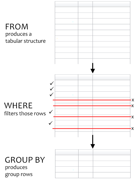
The GROUP BY clause fits into the context of the overall query right after the WHERE clause. Syntactically, a query begins with the SELECT clause which we’ll cover in Chapter 7. Then comes the FROM clause, the WHERE clause, and then the GROUP BY clause. More importantly, however, is the sequence in which the query clauses are executed:

• The FROM clause determines the contents of the intermediate tabular result that the query starts with.

• The WHERE clause, if present, filters the rows of that tabular structure.

• The GROUP BY clause, if present, aggregates the remaining rows into groups.

This is illustrated in Figure 5.6.

When a GROUP BY clause is present in the query, it aggregates many rows into one. After this is done, all the original rows produced by the FROM clause that survived the WHERE filter, are removed. The GROUP BY clause produces group rows, which you’ll recall from Chapter 2 are new rows created to represent each group of rows found during the aggregation process. The original rows are no longer available to the query. Only group rows come out of the grouping process.

Group Rows

One way to think about the grouping process goes like this:

• The FROM clause produces a temporary result set, held as a temporary table within the memory of the database system while the query is being executed.

• If a WHERE clause is present, only some of those rows will be retained. If a row passes the WHERE clause criteria, it is copied to a second temporary table. The second temporary table would still have the same tabular structure as the first one.

• If a GROUP BY clause is present, another temporary table is created for the group rows. This would have a different tabular structure from those produced by the FROM or WHERE clauses.

To see this process one more time, let’s look at another grouping example. Here again is the query from the previous example, but with an added WHERE condition:

Cart_11_GROUP_BY_WITH_WHERE.sql (excerpt)

SELECT 
  customers.name        AS customer
, SUM(cartitems.qty)    AS qty
, SUM(cartitems.qty
      * items.price)    AS total
FROM 
  customers 
    INNER JOIN carts
      ON carts.customer_id = customers.id
    INNER JOIN cartitems
      ON cartitems.cart_id = carts.id 
    INNER JOIN items
      ON items.id = cartitems.item_id
WHERE 
  items.name = 'thingum'
GROUP BY 
  customers.name 

The purpose of this query is to produce totals for each customer, but only for items called thingum. Thus, rather than seeing how many carts each customer has, we’re more interested in how many thingums were purchased. Remember the context of GROUP BY in the overall query. The GROUP BY clause operates after the WHERE clause, on the filtered intermediate tabular result, so we know that only thingum rows will be grouped. Notice also that in this query, instead of counting items in the customer carts, the qty result column in the SELECT clause is SUM(cartitems.qty), the total quantity of items.

Figure 5.7 shows the results:

Figure 5.7. Thingum purchases grouped by customer

Note: Aggregate Functions and GROUP BY

In the various preceding examples, different aggregate functions were used to produce different kinds of totals—number of carts, number of items, total quantity, total cost—while different GROUP BY clauses were used to produce aggregates at different levels.

We’ll discuss aggregate functions again in Chapter 7. For now, we need only to be aware that aggregate functions are often used in GROUP BY queries, to produce the kinds of totals—sums, counts, and so on—that we would expect them to from their function names.

As we’ve seen, the GROUP BY clause performs an aggregation on the rows produced by the FROM clause, and this grouping process creates group rows. Group rows are not the same as rows from the tabular structure coming out of the FROM clause.

So the first rule for using the GROUP BY clause is that the result set can contain only columns specified in the GROUP BY clause, or aggregate functions, or any combinations of these. This rule will show up again when we discuss the SELECT clause in Chapter 7.

Actually, columns in group rows can also include constants, as well as expressions built by combining GROUP BY columns, aggregate functions, and constants. But this nuance is inconsequential to the main point: group rows can contain only columns that are mentioned in the GROUP BY clause or are contained inside aggregate functions (or expressions built from these). The grouping process produces only these two column types.

Columns with Certain Large Data Types

Another point about using GROUP BY is that only some database systems let you specify columns with large data types in a GROUP BY clause. These particular data types, Binary Large Objects (BLOBs), and Character Large Objects (CLOBs), are covered in more detail in Chapter 9. Just quickly though, CLOBs are used to store large amounts of character data, while BLOBs are used to store binary data, such as images, sound, and video.

The restriction depends on the specific database system you’re using. However, it’s unnecessary to specify a BLOB or CLOB column in the GROUP BY clause in the first place. This is the direct consequence of a strategy I call pushing down the GROUP BY clause into a subquery whenever possible. The following example will illustrate this process.

In Chapter 2, we briefly encountered the Content Management System sample application. The CMS application is described in detail in the section called “Content Management System” in Appendix B. The entries table holds the entries that are the basis for our CMS. An entry has a title, date created, and so on. It also may have a large block of actual content. In the model of the CMS application (shown in Figure 5.8—more on these diagrams in the section called “Entity–Relationship Diagrams” in Chapter 10), this content is stored separately in a related row in the contents table. (In Chapter 2, the content column was actually in the entries table.)

Figure 5.8. The structure of the CMS database

Each row in the entries table has, at most, one row in the contents table, but could have none, because content is optional in our CMS. So, if we were to write a query to return the entries in our CMS, along with the content for each entry (if any), our query would look like this:

CMS_14_Content_and_Comment_tables.sql (excerpt)

SELECT 
  entries.id
, entries.title
, entries.created
, contents.content
FROM 
  entries
    LEFT OUTER JOIN contents
      ON contents.entry_id = entries.id

This is a straightforward left outer join; all entries are returned, including their related content, if any. If an entry has no matching contents row, then the row in the result set for that entry will have NULL in the content column.

But we’ve still to reach where the GROUP BY complexity comes into play. To do so, we need another table to join to—the comments table. Besides having an optional content row, each row in the entries table also has one or more optional rows in the comments table. Multiple comments can be made against each entry. In addition to returning each entry with its optional content, we want also to return a count of the number of comments for that entry.

Here’s the first attempt at the query to do this:

CMS_14_Content_and_Comment_tables.sql (excerpt)

SELECT 
  entries.id
, entries.title
, entries.created
, contents.content 
, COUNT(comments.entry_id) AS comment_count
FROM 
  entries
    LEFT OUTER JOIN contents
      ON contents.entry_id = entries.id
    LEFT OUTER JOIN comments
      ON comments.entry_id = entries.id
GROUP BY 
  entries.id
, entries.title
, entries.created
, contents.content

Let's take a look at the changes. First of all, the SELECT clause contains an aggregate function. The COUNT function will count the number of comments for each entry. However, we need a GROUP BY clause in order to do this, because a GROUP BY clause is what collapses the multiple comments rows into one, so that the COUNT function will work correctly.

Notice that the GROUP BY clause lists exactly the same columns as the columns in the SELECT clause. We want to return those columns in the query results, but in a GROUP BY query, only group row columns may be specified in the SELECT clause outside of aggregate functions. Therefore those columns have to be in the GROUP BY clause.

This would all be wonderful, if it actually ran. Unfortunately, contents.content is a TEXT column, another large data type like CLOB which—as noted earlier—some database systems won’t let you have in the GROUP BY clause.

There are two ways to work around this limitation, both involving a subquery.

The first solution is to push down the grouping process into a subquery, and then join this subquery into the query as a derived table, in place of the original table:

CMS_14_Content_and_Comment_tables.sql (excerpt)

SELECT
  entries.id
, entries.title
, entries.created
, contents.content 
, c.comment_count
FROM 
  entries
    LEFT OUTER JOIN contents
      ON contents.entry_id = entries.id
    LEFT OUTER JOIN ( 
      SELECT 
        entry_id 
     ,  COUNT(*) AS comment_count
     FROM
       comments
     GROUP BY
       entry_id
    ) AS c 
      ON c.entry_id = entries.id

Notice that in the derived table subquery, the GROUP BY clause specifies the entry_id. If there are multiple rows in the comments table for any entry_id, they are aggregated by the GROUP BY. Thus, the derived table consists of only group rows, which have only the entry_id and comment_count columns. The derived table therefore, has only one row per entry_id, and this is the column used to join the derived table to the entries table. The outer query no longer has a GROUP BY clause; it’s been pushed down into a subquery.

The second solution is similar, but instead of a subquery as a derived table in the FROM clause, it uses a correlated subquery in the SELECT clause:

CMS_14_Content_and_Comment_tables.sql (excerpt)

SELECT 
  entries.id
, entries.title
, entries.created
, contents.content 
, (
    SELECT 
      COUNT(entry_id)
    FROM
      comments
    WHERE
      entry_id = entries.id
  ) AS comment_count  
FROM 
  entries
    LEFT OUTER JOIN contents
      ON contents.entry_id = entries.id

We first discussed correlated subqueries back in the section called “Correlated Subqueries” in Chapter 4. The above solution omits the GROUP BY clause, yet it produces the same result. Once again, we see that there’s often more than one way to write an SQL query to achieve the results we want.

In fact, there is grouping in the above correlated subquery, but it’s implicit. We’ll explore this concept in the section called “Aggregate Functions without GROUP BY” in Chapter 7, but for now all you need to know is that when there’s only aggregate functions in the SELECT clause, like the COUNT(entry_id) aggregate function above, all of the rows returned by the FROM clause are considered to be one group. The effect of this, in the above query, is that the subquery produces an aggregate count of all correlated rows from the comments table for each id in the entries table from the outer query.

In this chapter, we learned about the concept of grouping.

In Chapter 6, we’ll meet the companion to the GROUP BY clause, the HAVING clause.