
Chapter 10
Sampling Theory
In This Chapter
![]() Getting the gist of sampling
Getting the gist of sampling
![]() Working with the ADC for periodic sampling
Working with the ADC for periodic sampling
![]() Checking out the sampling theory view in the frequency domain
Checking out the sampling theory view in the frequency domain
![]() Using the low-pass sampling theorem
Using the low-pass sampling theorem
![]() Avoiding aliasing with an antialiasing filter
Avoiding aliasing with an antialiasing filter
![]() Returning to the continuous-time using a DAC plus an interpolation filter
Returning to the continuous-time using a DAC plus an interpolation filter
The discrete-time signals you deal with in the real world often occur as a result of periodic (uniform) sampling of continuous-time signals. I’m talking about speech signals going into a cellphone, music signals captured in a recording studio, sensor signals in your car, radio signals in wireless devices, and the like. In this chapter, I describe the fundamentals of sampling theory and show you that designing a sampling system that allows for accurate reconstruction of a continuous-time signal from only discrete-time samples isn’t too difficult.
 Basically, sampling theory is the mathematics that explains the details of the signal-conversion process to and from the discrete-time domain. In the study of sampling theory, using the time-domain view (see Chapter 3) and the frequency-domain view (explored in Chapter 9) can help you get a handle on the underlying mathematics.
As this chapter unfolds, I cover the reconstruction filter, the antialiasing filter, and the quantizer, which is internal to the analog-to-digital converters (ADC). But the main focus is periodic sampling of a continuous-time signal to create a discrete-time signal. The sample values are taken as real (infinite precision) numbers for the most part — I pretty much ignore the bit width of the ADC; however, I briefly consider finite precision effects before presenting the frequency-domain view.
If you’re curious about the various ADC/DAC technologies available, search the web for “successive approximation register (SAR),” “delta-sigma (![]() ),” and “flash ADCs.”
),” and “flash ADCs.”
Seeing the Need for Sampling Theory
All the great attributes of discrete-time signals and systems rely on the ability to interface with the continuous-time domain. Analog-to-digital converters (ADCs) and digital-to-analog converters (DACs) are the electronic subsystems that convert signals between continuous-time and discrete-time signal forms. To that end, Figure 10-1 shows a top-level depiction of how to implement the interface of these two subsystems. The various components in this figure (except the first block, the antialiasing fliter) are described throughout this chapter. Find out how to use the antialiasing filter to avoid alaising at the ADC at www.dummies.com/extras/signalsandsystems.
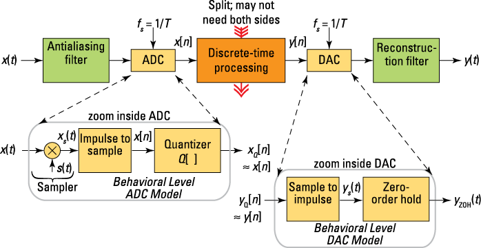
Figure 10-1: A block diagram showing how a discrete-time signal processing system (top center) interfaces with continuous-time signals, both input and output scenarios.
You want to process a continuous-time signal in the discrete-time domain to achieve better system performance and to enjoy the flexibility of a software-programmable solution. Some applications may require only the ADC and discrete-time processing. Other applications, such as a CD player, may need only the DAC side of the system.
The ADC converts ![]() to
to ![]() by using the sampling rate clock input
by using the sampling rate clock input ![]() . A discrete-time system processes
. A discrete-time system processes ![]() to produce output
to produce output ![]() . The discrete-time signal
. The discrete-time signal ![]() is converted back to continuous-time signal
is converted back to continuous-time signal ![]() via the DAC.
via the DAC.
At the heart of sampling theory is the minimum sampling rate, or one over the sample spacing, which is needed to ensure that the original continuous-time signal can be reconstructed from its samples.
Periodic Sampling of a Signal: The ADC
The ADC is responsible for converting the continuous-time (analog) signal ![]() into the corresponding discrete-time sequence
into the corresponding discrete-time sequence ![]() . From the ADC inset of Figure 10-1, follow these three steps to transform x(t) into a sequence of numbers corresponding to samples of x(t) taken at times nT, n the sample index.
. From the ADC inset of Figure 10-1, follow these three steps to transform x(t) into a sequence of numbers corresponding to samples of x(t) taken at times nT, n the sample index.
1. Take samples of ![]() by multiplying by an impulse train signal:
by multiplying by an impulse train signal:
![]()
The product ![]() remains a continuous-time signal because the waveform samples
remains a continuous-time signal because the waveform samples ![]() are still placed along the time axis. I explain why this is important in the next section on the frequency-domain view of sampling theory.
are still placed along the time axis. I explain why this is important in the next section on the frequency-domain view of sampling theory.
2. Convert the impulse train signal into a sequence of numbers:
![]()
In a real ADC, you can accomplish this step seamlessly via the electronics of the ADC. Here, keep in mind that the sequence values ![]() have infinite precision, as you may expect for a continuous-time signal.
have infinite precision, as you may expect for a continuous-time signal.
3. Quantize the sequence values ![]() . In other words, convert the infinite precision real number values to B-bit precision numbers.
. In other words, convert the infinite precision real number values to B-bit precision numbers.
B is an integer, which refers to the word length of the data type used to store the signal samples. In the notation of Figure 10-1, ![]() . The most common data type used for this purpose is the signed integer, which reserves one bit to convey sign information and B – 1 bits to convey the magnitude. For example, 16-bit signed integers range in value from
. The most common data type used for this purpose is the signed integer, which reserves one bit to convey sign information and B – 1 bits to convey the magnitude. For example, 16-bit signed integers range in value from ![]() to
to ![]() .
.
I cover the quantizer aspect of the ADC in the section “Analyzing the Impact of Quantization Errors in the ADC,” later in this chapter. Don’t worry: When B is large, ![]() . The net result of the idealized ADC is to produce
. The net result of the idealized ADC is to produce ![]() from the input
from the input ![]() .
.
 Example 10-1: Consider sampling the continuous-time sinusoid
 ![]() at sample spacing T or equivalently a sampling rate of
at sample spacing T or equivalently a sampling rate of ![]() . Here is the sampled signal
. Here is the sampled signal ![]() :
:
![]()
I use the notation ![]() for discrete-time frequency. Even though
for discrete-time frequency. Even though ![]() has units of radians, to emphasize the fact that sampling is involved, I prefer to think of the units as radians/sample. Because
has units of radians, to emphasize the fact that sampling is involved, I prefer to think of the units as radians/sample. Because ![]() , you can also define
, you can also define ![]() as the discrete-time frequency in cycles/sample.
as the discrete-time frequency in cycles/sample.
You may be wondering how many samples per period of ![]() are required. In Figure 10-2, I plot five scenarios of
are required. In Figure 10-2, I plot five scenarios of ![]() and
and ![]() for
for ![]() and
and ![]() , taking on four values. Here are the IPython command line entries for creating a single subplot of Figure 10-2.
, taking on four values. Here are the IPython command line entries for creating a single subplot of Figure 10-2.
In [412]: t = arange(0,10,.01)
In [413]: n = arange(0,11)
In [414]: plot(t,cos(2*pi*0.1*t)) # f0/fs = 0.1/1.0 = 0.1
In [415]: stem(n,cos(2*pi*0.1*n),'r','ro')
Figure 10-2a probably looks the nicest because it has ten samples per period. But looking nice isn’t of primary importance. The objective is to verify that you can reconstruct ![]() from the sample values .
from the sample values .
Figure 10-2b has only four samples per period, but it’s adequate. Figure 10-2c is too lean; both of the plots have just two samples per period. At only two samples per period, the plot shows that with proper phasing, ![]() , the samples become 0 everywhere. Not good!
, the samples become 0 everywhere. Not good!
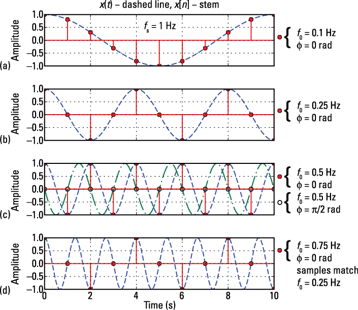
Figure 10-2: Sampling a 0.1 (a), 0.25 (b), 0.5 (c), and 0.75 (d) Hz sinusoid at a fixed rate of 1 Hz.
The low-pass sampling theorem, which I cover in the later section “Applying the Low-Pass Sampling Theorem,” states that fs must be greater than twice the highest frequency contained in x(t) to ensure reconstruction of ![]() from its samples. For the case of a single sinusoid, this is equivalent to fs > 2f0 or greater than two samples per period. Only Figures 10-2a and 10-2b satisfy this condition.
from its samples. For the case of a single sinusoid, this is equivalent to fs > 2f0 or greater than two samples per period. Only Figures 10-2a and 10-2b satisfy this condition.
Figure 10-2d, ![]() Hz, has fewer than two samples per period (
Hz, has fewer than two samples per period (![]() ) and the sample values match those of Figure 10-2b, where
) and the sample values match those of Figure 10-2b, where ![]() Hz. To find out what’s going on, look at the math behind the sequence plot, bearing in mind that cosine is a mod
Hz. To find out what’s going on, look at the math behind the sequence plot, bearing in mind that cosine is a mod![]() function:
function:

The 0.25-Hz and 0.75-Hz sinusoids produce the same sequence values when sampled at ![]() Hz. You can work with
Hz. You can work with ![]() values just as easily as frequency in hertz for this problem. Here are the equivalent radians/sample frequencies:
values just as easily as frequency in hertz for this problem. Here are the equivalent radians/sample frequencies:
![]()
The same result holds.
The ![]() nature of cosine is the key to making the frequency of the two real sinusoids equal in magnitude:
nature of cosine is the key to making the frequency of the two real sinusoids equal in magnitude: ![]() . The sign isn’t an issue here because Euler’s formula tells you that a real sinusoid is composed of positive and negative frequency complex sinsuoids, specifically
. The sign isn’t an issue here because Euler’s formula tells you that a real sinusoid is composed of positive and negative frequency complex sinsuoids, specifically
![]()
In this case, however, the cosine is even and ![]() , so the sample values are identical, as Figures 10-2b and 10-2c show. The fact that two single sinusoid signals, at frequencies 0.5 and 1.5 Hz, when sampled at 1 Hz have the same discrete-time frequency,
, so the sample values are identical, as Figures 10-2b and 10-2c show. The fact that two single sinusoid signals, at frequencies 0.5 and 1.5 Hz, when sampled at 1 Hz have the same discrete-time frequency, ![]() , represents aliasing. And, when aliasing is present, you don’t know the true frequency of the original input signal x(t). If the input to the ADC isn’t protected with an antiliasing filter (see the section “Using an Antialiasing Filter to Avoid Aliasing at the ADC”) the true signal frequency can’t be discovered.
, represents aliasing. And, when aliasing is present, you don’t know the true frequency of the original input signal x(t). If the input to the ADC isn’t protected with an antiliasing filter (see the section “Using an Antialiasing Filter to Avoid Aliasing at the ADC”) the true signal frequency can’t be discovered.
If ![]() in Example 10-1 is nonzero, then the following two expressions exist for sample equality, depending on the sign of
in Example 10-1 is nonzero, then the following two expressions exist for sample equality, depending on the sign of ![]() :
:
![]()
Here, ![]() and so on, and n is arbitrary. The smallest value
and so on, and n is arbitrary. The smallest value ![]() is called the principle alias.
is called the principle alias.
Assuming ![]() is the principle alias, the remaining alias frequencies in radians/sample are
is the principle alias, the remaining alias frequencies in radians/sample are ![]() ,
, ![]() and so on. In terms of continuous-time frequencies in hertz, the principle alias lies on the interval
and so on. In terms of continuous-time frequencies in hertz, the principle alias lies on the interval ![]() . Given f is the principle alias, the remaining alias frequencies in hertz are
. Given f is the principle alias, the remaining alias frequencies in hertz are ![]() , k = 1, 2, 3 and so on.
, k = 1, 2, 3 and so on.
 You can get a graphical view of the aliased frequencies by using a strip of paper folded like an accordian. As shown in Figure 10-3, the strip represents the continuous-time frequency axis, f, and the folds in the strip occur at multiples of
 ![]() .
.
The principle alias range is at the far left of Figure 10-3. Horizontal lines join together and collapse the common alias frequencies onto the principle alias or vice versa. The first fold point, ![]() , is the folding frequency.
, is the folding frequency.
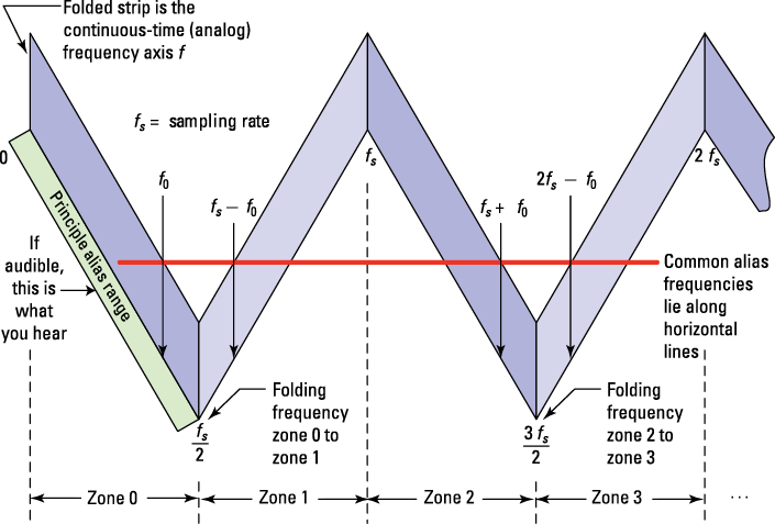
Figure 10-3: 3D depiction of the aliased frequencies via a folded strip of paper.
Figure 10-3 also shows alias zones as the contiguous frequency bands of length ![]() , starting with the principle alias band. Each zone always contains exactly one of the alias frequencies. The horizontal line confirms this.
, starting with the principle alias band. Each zone always contains exactly one of the alias frequencies. The horizontal line confirms this.
When you need to find the principle alias given the sampling rate and input frequency f, this formula comes in handy:
![]()
This formula is fast and efficient, but I also highly recommend spending time with the core relationship ![]() , where k is a nonnegative integer. Finding alias frequencies f given fprinciple is no problem; just pick a value for k.
, where k is a nonnegative integer. Finding alias frequencies f given fprinciple is no problem; just pick a value for k.
But when you’re given f and need to find fprinciple, you need to first find k such that f is within ![]() of kfs. From Figure 10-3, choosing k sets up a pair of contiguous alias zones with kfs at the center. For k = 1, you see whether f lies in Zones 1 or 2, for k = 2, Zones 3 and 4, and so on. After you find k, the principle alias frequency follows from the core relationship and Figure 10-3 as
of kfs. From Figure 10-3, choosing k sets up a pair of contiguous alias zones with kfs at the center. For k = 1, you see whether f lies in Zones 1 or 2, for k = 2, Zones 3 and 4, and so on. After you find k, the principle alias frequency follows from the core relationship and Figure 10-3 as ![]() . Note that f0 in Figure 10-3 is fprinciple.
. Note that f0 in Figure 10-3 is fprinciple.
To develop the formula for ![]() , start working backward from the formula for the alias frequencies:
, start working backward from the formula for the alias frequencies: ![]() .
.
To find k, an integer, such that ![]() is within
is within ![]() of f and as close to f as possible, choose
of f and as close to f as possible, choose ![]() . The absolute value of the difference between
. The absolute value of the difference between ![]() and f is then
and f is then ![]() .
.
Example 10-2: Consider an ADC (sampler) with ![]() kHz and a single sinusoid input signal. To begin the process of finding the principle alias frequency associated with the input frequencies: (a) 3, (b) 11, (c) 36, and (d) 122 kHz, start with what you know. The principle alias frequency band is [0, 5] kHz, so now find the principle alias for each frequency, using the core equation and the handy formula
kHz and a single sinusoid input signal. To begin the process of finding the principle alias frequency associated with the input frequencies: (a) 3, (b) 11, (c) 36, and (d) 122 kHz, start with what you know. The principle alias frequency band is [0, 5] kHz, so now find the principle alias for each frequency, using the core equation and the handy formula ![]() as a check. There are four parts to this problem; they’re labeled a–d in this process.
as a check. There are four parts to this problem; they’re labeled a–d in this process.
Using the core equation takes two steps:
1. Find k such that f is within ![]() of kfs.
of kfs.
2. Compute fprinciple as ![]() .
.
a. The 3-kHz signal is the principle alias already because it lies on the interval [0, 5] kHz. As a check, ![]() kHz.
kHz.
The two closest alias frequencies to 3 kHz are when k = 1: ![]() kHz and
kHz and ![]() kHz.
kHz.
b. The 11-kHz signal clearly isn’t a principle alias because it lies outside the interval [0, 5] kHz. From Step 1, find k that places 11 kHz within 10/2 = 5 KHz on either side of ![]() KHz. Setting k = 1 works. Applying Step 2
KHz. Setting k = 1 works. Applying Step 2 ![]() kHz. Using the formula,
kHz. Using the formula, ![]() kHz.
kHz.
c. For the 36-kHz signal, Step 1 says choose k to make 36 kHz within 5 KHz of k · 10, which means k = 4, because 40 KHz is only 4 kHz above 36 kHz. Applying Step 2, ![]() kHz. Using the formula,
kHz. Using the formula, ![]() kHz.
kHz.
d. With f = 122 kHz, Step 1 again requires f to be within 5 kHz of ![]() . As a guess, 122/10 = 12.2 and
. As a guess, 122/10 = 12.2 and ![]() . So k = 12 works because 122 is only 2 kHz away from 120 kHz. Applying Step 2,
. So k = 12 works because 122 is only 2 kHz away from 120 kHz. Applying Step 2, ![]() kHz. Using the formula,
kHz. Using the formula, ![]() kHz.
kHz.
Example 10-3: To find the principle alias, using PyLab, you can write a one-line function in IPython to work with numpy vectors (also included in ssd.py).
In [578]: def prin_alias(f_in,fs):
...: return abs(rint(f_in/fs)*fs - f_in)
Test the function by using the four frequency values of Example 10-2:
In [579]: ssd.prin_alias(array([3,11,26,122]),10.)
Out[579]: array([ 3., 1., 4., 2.])
The Python numerical results agree with the answers found in Example 10-2.
Analyzing the Impact of Quantization Errors in the ADC
The quantizer, ![]() , present in the ADC drill down of Figure 10-1, has a practical function. The ideal sampler (covered in the section “Periodic Sampling of a Signal: The ADC,” earlier in this chapter) forms samples of the continuous-time waveform
, present in the ADC drill down of Figure 10-1, has a practical function. The ideal sampler (covered in the section “Periodic Sampling of a Signal: The ADC,” earlier in this chapter) forms samples of the continuous-time waveform ![]() . The sample values themselves require infinite precision to be stored error-free on a computer. The quantizer rounds (or perhaps truncates) the signal sample to a finite precision binary word of B bits:
. The sample values themselves require infinite precision to be stored error-free on a computer. The quantizer rounds (or perhaps truncates) the signal sample to a finite precision binary word of B bits:
![]()
In signals and systems work, you typically use a bipolar quantizer where input x is rounded to the nearest quantization level xq, which takes on values ranging from ![]() to
to ![]() , where
, where ![]() is the step size defined as
is the step size defined as ![]() .
.
The quantization levels aren’t symmetrical about zero because 2B is even and a level needs to appear at zero. Note also that the output saturates, meaning that inputs outside the quantization range are held at the minimum and maximum quantization levels.
You need to know your limitations when working with an ADC; don’t input signals that exceed ![]() or suffer the consequences of larger error between the input and output. The input/output relationship for a B = 5 bit quantizer (B2 = 32 levels) is shown in Figure 10-4.
or suffer the consequences of larger error between the input and output. The input/output relationship for a B = 5 bit quantizer (B2 = 32 levels) is shown in Figure 10-4.

Figure 10-4: The input/output characteristic for a bipolar quantizer, using rounding and having B = 5 bits.
In practical systems, B runs from about 8 to 24. CD digital audio uses at minimum 16 bits per sample.
Samples x(nT) have infinite precision, but following the quantizer error is introduced due to the B-bit precision imposed by Q( ). The signal ![]() is known as the quantization error. With rounding and a step size of
is known as the quantization error. With rounding and a step size of ![]() , the quantization error ranges over
, the quantization error ranges over ![]() .
.
You can view e[n] as an additive noise source by rearranging the definition: ![]() . Using this arrangement, the error signal is referred to as quantization noise, because it appears as a noise-like signal being added to the infinite precision signal x(nT). I say noise-like because e[n] is functionally related to x(nT). You measure the impact of quantization noise by the ratio of power in x(nT) over the power in e[n]. It can be shown that for x(t), a sinusoid of amplitude Xm the signal-to-quantization noise ratio (SNRQ) in dB is approximately 6.02B + 1.76. For CD audio quality audio (B = 16), something you’re familiar with, this works out to 98 dB. Very good!
. Using this arrangement, the error signal is referred to as quantization noise, because it appears as a noise-like signal being added to the infinite precision signal x(nT). I say noise-like because e[n] is functionally related to x(nT). You measure the impact of quantization noise by the ratio of power in x(nT) over the power in e[n]. It can be shown that for x(t), a sinusoid of amplitude Xm the signal-to-quantization noise ratio (SNRQ) in dB is approximately 6.02B + 1.76. For CD audio quality audio (B = 16), something you’re familiar with, this works out to 98 dB. Very good!
You can use the Python function simpleQuant(x,Btot,Xmax,Limit) (in ssd.py) to quantize a sinusoid that falls inside the ![]() dynamic range of the quantizer. Find the experimental SNRQ, using the function
dynamic range of the quantizer. Find the experimental SNRQ, using the function var() to estimate the power in x(nT) and e[n] and then forming the power ratio. Here, I plot the error signal waveform in Figure 10-5.
In [38]: n = arange(0,10000)
In [39]: x = 0.99*cos(2*pi*n/11.23)# < Xm - delta
In [40]: xQ = ssd.simpleQuant(x,8,1,'sat') # quantize x
In [43]: plot(n,xQ-x) # plot the error signal
In [158]: 10*log10(var(xQ)/var(xQ-x)) # Exp. SNRQ in dB
Out[158]: 49.70
In [159]: 6.02*8+1.76 # Theory SNRQ in dB
Out[159]: 49.92
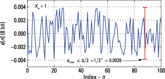
Figure 10-5: Quantizer error signal (a) and quantized signal spectrum (b) for B = 8 bits.
The peak quantization error lies within ![]() as expected. For 8 bits, the SNRQ is about
as expected. For 8 bits, the SNRQ is about ![]() dB, compared with 49.7 dB from the Python simulation.
dB, compared with 49.7 dB from the Python simulation.
Analyzing Signals in the Frequency Domain
Fourier transform theory really shines as a means to understand how to make sampling theory work for you. In this section, I develop a frequency-domain view of sampling theory. You need to understand the Fourier transform (FT) to get a handle on this material, so flip to Chapter 9 if you need to refresh your FT skills.
The first step in getting to frequency-domain view of sampling theory is to establish the spectrum of the input signal following multiplication by an ideal sampling waveform. The operation models the first stage of the ADC shown in Figure 10-1.
With a model for the sampled signal spectrum in hand, I can show you what the spectrum of a sampled bandlimited signal looks like. The corresponding spectral plot allows you to see how to avoid aliasing and what the consequences are if you don’t choose a large enough sampling rate — the aliased or folded spectrum occurs when the sampling rate is too small. Aliasing is most clearly visible in the frequency domain.
Impulse train to impulse train Fourier transform theorem
The spectral view of sampling theory isn’t limited to sinusoidal signals; it can handle all sorts of practical signals. In this section, I explore sampling theory in the frequency domain by developing the FT of an ideal impulse train sampled signal, which is generated inside the first stage of ADC model (refer to Figure 10-1). Intentionally allowing aliasing to occur, a topic not covered in this book, can be well-appreciated in the spectrum of the impulse train sampled signal.
The goal here is to get ![]() the spectrum of sampled signal
the spectrum of sampled signal ![]() . To start, find
. To start, find ![]() .
.
Because an impulse train in the time domain is an impulse train in the frequency domain, you can write this equation:
![]()
Now, convolve an impulse train in frequency with ![]() . To complete the term-by-term convolution, you need to know that a basic property of the impulse function and convolution is
. To complete the term-by-term convolution, you need to know that a basic property of the impulse function and convolution is ![]() (see Chapter 5).
(see Chapter 5).
Putting it all together,
![]()
This says that the spectrum of a sampled signal is a superposition of the original signal spectrum (![]() ) plus spectral translates — refers to frequency shifting X(f) by f0 to produce X(f – f0) — with translation offsets
) plus spectral translates — refers to frequency shifting X(f) by f0 to produce X(f – f0) — with translation offsets ![]() integer multiples of the sampling rate.
integer multiples of the sampling rate.
This is a cool and powerful result because it shows that Xs(f) contains the desired spectrum X(f) surrounded by its frequency translates. It also reveals that altering fs makes the picture either clear or cluttered (if you can’t wait, take a peek at the figures in the next section).
The result is somewhat counterintuitive because, in the time domain, sampling gives you less than what you started with (just the samples), but you have more in the frequency domain — the original spectrum X(f) plus all the translates ![]() and so on. Usually, the desire is to recover X(f) without capturing any of the spectral translates.
and so on. Usually, the desire is to recover X(f) without capturing any of the spectral translates.
Finding the spectrum of a sampled bandlimited signal
Suppose that ![]() has bandlimited spectrum of the form
has bandlimited spectrum of the form ![]() .
.
The sampled signal spectrum is

Figure 10-6 shows plots of ![]() and
and ![]() for
for ![]() and
and ![]() .
.
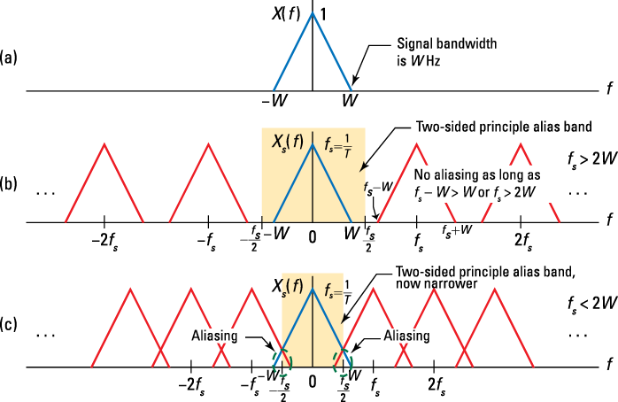
Figure 10-6: The spectra of a bandlimited signal: before sampling (a), after sampling with fs > 2W (b), and after sampling with fs < 2W (c).
When ![]() , all the spectral translates are distinct, meaning no overlap occurs between them. The principle translate, which in this book is always centered on
, all the spectral translates are distinct, meaning no overlap occurs between them. The principle translate, which in this book is always centered on ![]() , is the one you want to keep your eyes on here, because it corresponds to
, is the one you want to keep your eyes on here, because it corresponds to ![]() to within a scale factor. When
to within a scale factor. When ![]() , neighbors infringe upon the principle translate. The overlap is aliasing as it appears in the frequency domain.
, neighbors infringe upon the principle translate. The overlap is aliasing as it appears in the frequency domain.
I’ve been using frequency f in hertz so far in my explanations of the sampled signal spectrum, but you may need other units at some point in your signals and systems studies or work. You can plot the spectra by using ![]() or, in terms of the discrete-time frequency variable,
or, in terms of the discrete-time frequency variable, ![]() . To make this clear, Figure 10-7 is the spectrum of
. To make this clear, Figure 10-7 is the spectrum of ![]() , as shown in Figure 10-6b, with addition of two parallel frequency axes.
, as shown in Figure 10-6b, with addition of two parallel frequency axes.
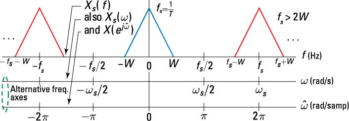
Figure 10-7: The sampled signal spectra, using alternative frequency axes.
The first two axes follow directly from ![]() and the two forms of the Fourier transform as I describe in Chapter 9. Using
and the two forms of the Fourier transform as I describe in Chapter 9. Using ![]() as a frequency axis suggests that
as a frequency axis suggests that ![]() has a Fourier transform (FT) representation, too. If you’re interested in the details of developing the proof for
has a Fourier transform (FT) representation, too. If you’re interested in the details of developing the proof for ![]() , check out Chapter 11. In the remainder of this chapter, you can assume that
, check out Chapter 11. In the remainder of this chapter, you can assume that ![]() exists and, with the change of variables
exists and, with the change of variables ![]() , the spectra of
, the spectra of ![]() are identical.
are identical.
Example 10-4: To find the sampled spectrum ![]() for
for ![]() , use the transform pair
, use the transform pair ![]() for X(f).
for X(f).
Plug into the sampled spectrum formula:
![]()
Now, plot the spectrum for ![]() , taking on values of 30 Hz and then 15 Hz. (Figure 10-8 shows this plot.)
, taking on values of 30 Hz and then 15 Hz. (Figure 10-8 shows this plot.)
To simplify the creation of the figure itself, you can use a custom function lp_samp(fb,fs,fmax,N,shape) written in Python to create the spectrum picture. The function code is available at www.dummies.com/extras/signalsandsystems in the module ssd.py, and it can make plots similar to Figures 10-6 and 10-7 when shape = 'tri' as well as a line spectra plot when shape = 'line'.
The parameter fb is equivalent to W when the triangle shape is used and f0 for the single sinusoid. The sampling rate is set via fs; fmax controls the frequency extent of the plot and N, the number of spectral translates to plot. Now create plots for the two fs values:
In [589]: ssd.lp_samp(10,30,60,5,'line')
In [592]: ssd.lp_samp(10,15,60,5,'line')
With ![]() Hz, fs needs to be greater than 20 Hz. With
Hz, fs needs to be greater than 20 Hz. With ![]() Hz, aliasing is visible.
Hz, aliasing is visible.
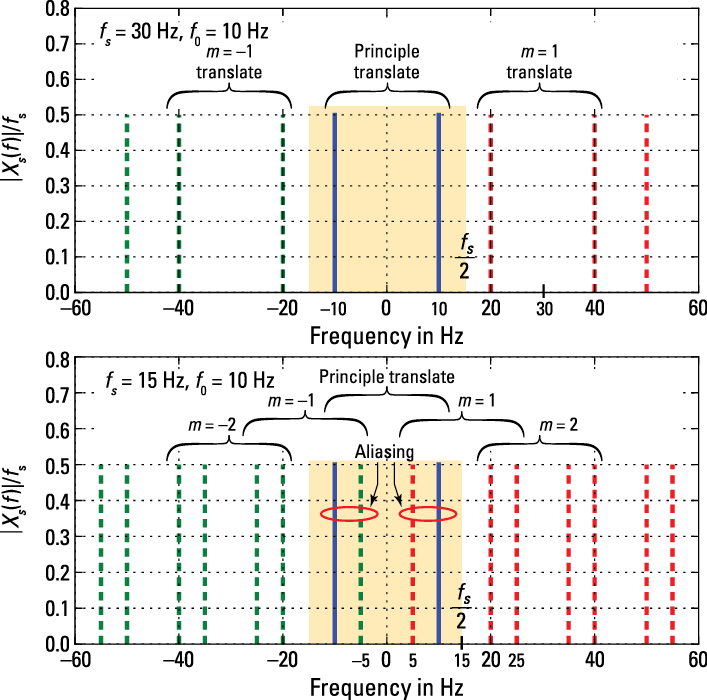
Figure 10-8: The sampled signal spectrum for a single 10-Hz sinusoid for a sampling rate of 30 Hz (a) and 15 Hz (b).
Sure enough, when you sample the 10-Hz sinusoid at 15 Hz, an alias spectral line falls below the principle translate at 5 Hz. The principle alias formula ![]() agrees because
agrees because ![]() Hz.
Hz.
Aliasing and the folded spectrum
The spectral translate at ![]() , given by
, given by ![]() , is centered on
, is centered on ![]() because X(f) is assumed symmetrical about f = 0. The spectrum tail that laps below
because X(f) is assumed symmetrical about f = 0. The spectrum tail that laps below ![]() appears to be a folded version of the principle translate that lies above
appears to be a folded version of the principle translate that lies above ![]() . This is depicted graphically in Figure 10-9.
. This is depicted graphically in Figure 10-9.
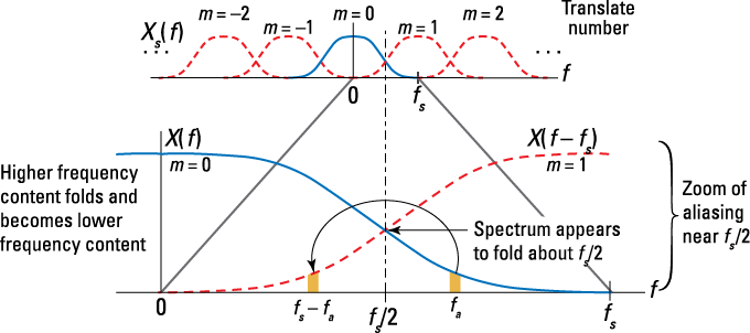
Figure 10-9: The folded spectrum that results from the m = 1 spectral translate lapping below ![]() .
.
The symmetry evident about ![]() earns the half sampling rate frequency the name folding frequency. Suppose that
earns the half sampling rate frequency the name folding frequency. Suppose that ![]() kHz and
kHz and ![]() contains a spectral component at 1,200 Hz. The spectrum folding action of Figure 10-9 places an aliased spectral component at 800 Hz. Why? Symmetry about 1,000 Hz demands that the 1,200-Hz component fold to 200 Hz below 1,000 Hz, which is 800 Hz.
contains a spectral component at 1,200 Hz. The spectrum folding action of Figure 10-9 places an aliased spectral component at 800 Hz. Why? Symmetry about 1,000 Hz demands that the 1,200-Hz component fold to 200 Hz below 1,000 Hz, which is 800 Hz.
Don’t worry: I haven’t violated the principle alias formula. From the given information, ![]() Hz, which indicates that a signal at 1,200 Hz has a principle alias frequency of 2,000 – 1,200 = 800 Hz. The folded spectrum is just another way of looking at the inner workings of sampling theory.
Hz, which indicates that a signal at 1,200 Hz has a principle alias frequency of 2,000 – 1,200 = 800 Hz. The folded spectrum is just another way of looking at the inner workings of sampling theory.
Applying the Low-Pass Sampling Theorem
When ![]() (as it is in Figure 10-6c), the band of frequencies
(as it is in Figure 10-6c), the band of frequencies ![]() contains only the principle (
contains only the principle (![]() ) translate. This translate is simply an amplitude scaled version of the original spectrum
) translate. This translate is simply an amplitude scaled version of the original spectrum ![]() . To recover
. To recover ![]() from
from ![]() , all you need to do is pass
, all you need to do is pass ![]() through an ideal low-pass filter (see Chapter 9) that keeps the principle translate and discards everything else. In mathematical terms,
through an ideal low-pass filter (see Chapter 9) that keeps the principle translate and discards everything else. In mathematical terms,
![]()
Here, ![]() is the impulse response of an ideal low-pass filter having bandwidth (or cutoff frequency)
is the impulse response of an ideal low-pass filter having bandwidth (or cutoff frequency) ![]() . Note that
. Note that ![]() . If
. If ![]() recovery isn’t possible because of the presence of aliasing inside the band of frequencies, then
recovery isn’t possible because of the presence of aliasing inside the band of frequencies, then ![]() .
.
You can now formally state the low-pass sampling theorem:
![]() Let
Let ![]() be a bandlimited signal such that
be a bandlimited signal such that ![]() .
.
Recover ![]() from its samples
from its samples ![]() , provided that
, provided that ![]() .
.
![]() W is referred to as the Nyquist frequency.
W is referred to as the Nyquist frequency.
![]() 2W is the Nyquist rate.
2W is the Nyquist rate.
To find out how to use the antialising filter (the very first block in Figure 10-1) to block signals above the folding frequency, ![]() , from entering the ADC and thus avoid aliasing, check out
, from entering the ADC and thus avoid aliasing, check out www.dummies.com/extras/signalsandsystems.
Reconstructing a Bandlimited Signal from Its Samples: The DAC
I’ve said a lot about sampling a continuous-time signal. Now it’s time to focus on how to reconstruct a continuous-time signal from a sequence of samples. When you listen to a CD, talk on a cellphone, or stream music from Internet radio, a sequence of signal values converts back to an intact continuous-time signal to reach the speaker. This happens in two steps:
1. The device places the signal samples back on the physical time axis.
2. The device interpolates a continuum of signal values between the sample values.
Take a system, or behavioral, level view of these two steps. A circuit designer would treat this as a mixed signal design problem, which means that the circuit is composed of both digital logic and analog circuit (continuous-time) building blocks.
The zoom inside the DAC at the bottom right of Figure 10-1 shows you that the first step for converting the discrete-time signal ![]() to the continuous-time signal,
to the continuous-time signal, ![]() , is placing the sequence values on the time axis using time-shifted impulse functions:
, is placing the sequence values on the time axis using time-shifted impulse functions: ![]() . The DAC sampling rate clock, at frequency fs = 1/T, is used to establish the time spacing.
. The DAC sampling rate clock, at frequency fs = 1/T, is used to establish the time spacing.
Next, the impulse train signal passes through a zero-order hold (ZOH) operation. The ZOH models the output of a realizable DAC (a working design in electronic circuit form), where the output of each conversion cycle is held constant from one sample period to the next. This makes the output waveform resemble a set of stairs. The ZOH provides a conversion between the impulse train and the stairstep waveform. Viewed as a linear filter, the impulse response of the ZOH is ![]() .
.
The corresponding frequency response of the ZOH filter is ![]() . The ZOH output is the convolution of
. The ZOH output is the convolution of ![]() with
with ![]() :
:
![]()
Here, the sample values are placed every T seconds. Figure 10-10 shows the relation between the samples ![]() , the ZOH output, and the recovered/reconstructed output
, the ZOH output, and the recovered/reconstructed output ![]() .
.
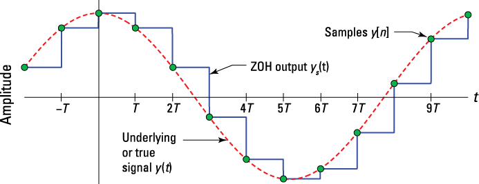
Figure 10-10: The DAC ZOH stairstep waveform and the associated input samples and perfectly reconstructed output.
The output of the ZOH needs additional filtering for ys(t) to approximate y(t), the true signal. The reconstruction filter has frequency response ![]() and an impulse response
and an impulse response ![]() . Getting the reconstructed output requires one more convolution:
. Getting the reconstructed output requires one more convolution:
![]()
Note that ![]() . The combination of both filters smoothly interpolates signal values between the original samples spaced at T. The low-pass filter is hr(t). I explore the details of hr(t) in the next two sections.
. The combination of both filters smoothly interpolates signal values between the original samples spaced at T. The low-pass filter is hr(t). I explore the details of hr(t) in the next two sections.
Interpolating with an ideal low-pass filter
In the absence of a DAC ZOH filter, the ideal reconstruction filter can be an ideal low-pass filter with gain T (to compensate for the ![]() gain from the sampling operation) and cutoff frequency
gain from the sampling operation) and cutoff frequency ![]() . The ideal low-pass filter has impulse response
. The ideal low-pass filter has impulse response ![]() (see Chapter 9).
(see Chapter 9).
You must deal with the impact of the ZOH filter before going any further. The ZOH sinc function frequency response introduces frequency droop over the frequency band ![]() . Frequency droop means that the frequency response magnitude rounds downward instead of being flat for frequencies between 0 and fs/2. See the plot in Figure 10-11.
. Frequency droop means that the frequency response magnitude rounds downward instead of being flat for frequencies between 0 and fs/2. See the plot in Figure 10-11.
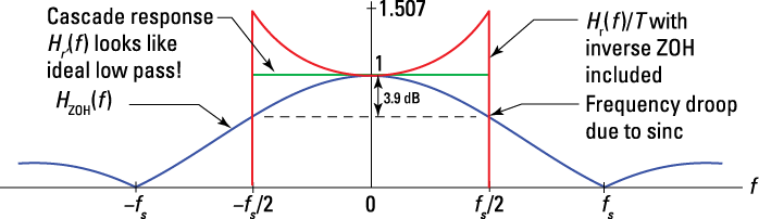
Figure 10-11: The frequency response of the ZOH filter and how to compensate for frequency droop with a compensator incorporated into ![]() .
.
To make the cascade response ![]() look like an ideal low-pass filter, with constant frequency response magnitude out to fs/2, you need to incorporate an inverse sinc function frequency response into Hr(f). Figure 10-11 shows how you can modify
look like an ideal low-pass filter, with constant frequency response magnitude out to fs/2, you need to incorporate an inverse sinc function frequency response into Hr(f). Figure 10-11 shows how you can modify ![]() so the cascade response looks like an ideal low-pass filter. The compensated Hr(f) is an ideal low-pass with the addition of a cup-shape amplitude response for
so the cascade response looks like an ideal low-pass filter. The compensated Hr(f) is an ideal low-pass with the addition of a cup-shape amplitude response for ![]() .
.
In practice, you can place the compensator in the discrete-time domain by using a simple digital filter or incorporate it into the reconstruction filter ![]() (see Chapter 15 for a digital filter design example).
(see Chapter 15 for a digital filter design example).
From this point forward, I assume that the compensation of the ZOH is already addressed. Keep in mind that some DAC chips make inverse sinc compensation totally transparent to the system designer.
To begin the ideal low-pass modeling process, write the time-domain formula for getting the recovered signal (assuming the ZOH is compensated):
![]()
The sinc function serves as an ideal interpolation function in this case because the impulse response is non-causal.
Example 10-5: In this example, I show you how the sinc interpolation function (the ideal low-pass reconstruction filter) creates y(t) from a finite set of sample values y[n]. In particular, I assume that y[n] is found by sampling ![]() with fs = 1 Hz. The available samples are limited to
with fs = 1 Hz. The available samples are limited to ![]() .
.
To show you the reconstruction process step by step, I first create an overlay plot in Figure 10-12a of the individual waveforms ![]() , corresponding to each available sample. The sample values are filled circles, and the original continuous-time sinusoid is a dashed line.
, corresponding to each available sample. The sample values are filled circles, and the original continuous-time sinusoid is a dashed line.
In Figure 10-12b, the individual waveform contributions are added together to form the composite or reconstructed output y(t).
Once inside the interpolation interval, the reconstruction is good, as evidenced by the two curves lying on top of each other.
Example 10-6: Consider an end-to-system that employs ideal sampling and ideal low-pass reconstruction. Assume that the discrete-time system placed between the ADC and DAC is a signal pass through, meaning ![]() .
.
The analog input signal is ![]() , and the sampling rate is 48 kHz. CD digital audio uses
, and the sampling rate is 48 kHz. CD digital audio uses ![]() kHz. The 48-kHz rate, and inter multiples thereof, are popular in recording studio audio processing.
kHz. The 48-kHz rate, and inter multiples thereof, are popular in recording studio audio processing.
Sketch the frequency spectra ![]() . The system block diagram is available in Figure 10-13.
. The system block diagram is available in Figure 10-13.
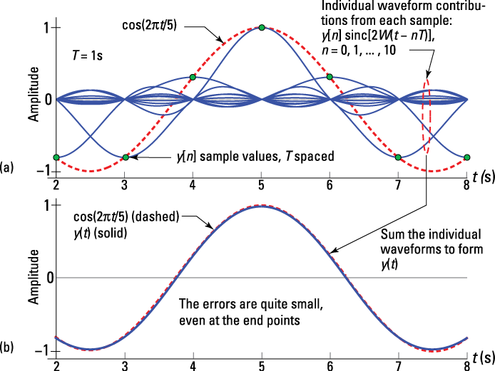
Figure 10-12: The ideal low-pass filter, via the sinc function, interpolates values between the y[n] samples and form y(t).
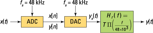
Figure 10-13: System block diagram for Example 10-6.
Before you jump into plotting anything, find out whether aliasing is present. Aliasing occurs for input frequencies above 24 kHz. The 10-kHz signal is fine, but the 36-kHz signal aliases to 48 – 36 = 12 kHz. After it’s inside the system, the 36 kHz signal loses its identity and becomes forever a 12-kHz signal. To find ![]() , use Fourier transform pair
, use Fourier transform pair ![]() to get the following:
to get the following:

The spectrum X(f) is sketched in Figure 10-14a. The spectrum ![]() , shown in Figure 10-14b, consists of
, shown in Figure 10-14b, consists of ![]() and translates
and translates ![]() scaled by
scaled by ![]() . When you use an ideal low-pass reconstruction filter (see overlay in Figure 10-14b), the output spectrum
. When you use an ideal low-pass reconstruction filter (see overlay in Figure 10-14b), the output spectrum ![]() consists of the spectrum content of
consists of the spectrum content of ![]() that lies in the two-sided principle alias band
that lies in the two-sided principle alias band ![]() . The spectrum Y(f) in Figure 10-14c shows that the 36-kHz sinusoid is aliased to 12 kHz, as expected.
. The spectrum Y(f) in Figure 10-14c shows that the 36-kHz sinusoid is aliased to 12 kHz, as expected.
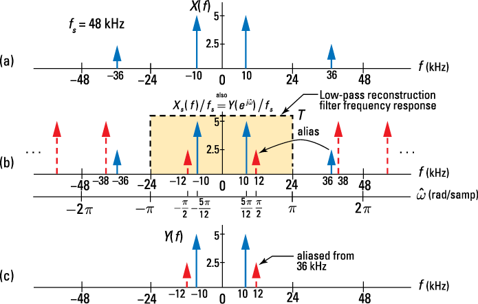
Figure 10-14: Sampling and then reconstructing 10- and 36-KHz sinusoids with fs = 48 kHz: input spectrum (a), sampled signal spectrum (b), and output spectrum with aliasing (c).
Using a realizable low-pass filter for interpolation
Assuming ![]() is bandlimited and
is bandlimited and ![]() is chosen to satisfy the low-pass sampling theorem, the filtering action of an ideal low-pass filter (shaded region in Figure 10-6b) perfectly extracts the principle spectral translate of Xs(f). In the time domain, the interpolation is perfect, too, because only
is chosen to satisfy the low-pass sampling theorem, the filtering action of an ideal low-pass filter (shaded region in Figure 10-6b) perfectly extracts the principle spectral translate of Xs(f). In the time domain, the interpolation is perfect, too, because only ![]() is returned at the filter output.
is returned at the filter output.
When using a realizable filter (see Chapter 9), the filter magnitude response doesn’t jump instantly to 0 for f >![]() . The magnitude response becomes very small only gradually as frequency increases, depending on the filter order you choose. This means that spectral translates for
. The magnitude response becomes very small only gradually as frequency increases, depending on the filter order you choose. This means that spectral translates for ![]() are present in the filter output. These translates are weak, but they’re still present, so the reconstructed output contains distortion — imperfect interpolation.
are present in the filter output. These translates are weak, but they’re still present, so the reconstructed output contains distortion — imperfect interpolation.
You can increase the filter order but only at the expense of increased complexity. To ease the filter design requirements, you can use oversampling, which involves setting ![]() to some integer factor greater than 2W, to provide an effective guard band of frequencies between the principle translate and its nearest neighbors. The guard band allows the filter magnitude response to roll off more before encountering the first spectral translate. To visualize the impact of oversampling, think of moving the
to some integer factor greater than 2W, to provide an effective guard band of frequencies between the principle translate and its nearest neighbors. The guard band allows the filter magnitude response to roll off more before encountering the first spectral translate. To visualize the impact of oversampling, think of moving the ![]() spectral translates in Figure 10-6b much farther away from the m = 0 translate.
spectral translates in Figure 10-6b much farther away from the m = 0 translate.
Oversampling in this fashion increases complexity. A popular oversampling technique is to increase the sampling rate (upsampling) in the discrete-time domain, just prior to the DAC. This way, low-pass reconstruction filtering can begin in the discrete-time domain at the oversampled rate by using an efficient digital filter.
The final stage of reconstruction filtering that takes place in the continuous-time domain then needs to be only a low-order analog filter. The downside is that the DAC must be clocked at a higher sampling rate. For audio signal processing used in consumer electronics, oversampling DACs are viable and thus used in devices you likely own.