
Chapter 7
LTI System Differential and Difference Equations in the Time Domain
In This Chapter
![]() Checking out LCC differential equation representations of LTI systems
Checking out LCC differential equation representations of LTI systems
![]() Exploring LCC difference equations
Exploring LCC difference equations
A special class of LTI systems contains systems that have linear constant coefficient (LCC) differential or difference equation representations in the continuous- or discrete-time domains, respectively. (Find general information about LTI systems in the time domain in Chapters 5 and 6.)
 One thing to know right off the bat here is that the abbreviation LCCDE often applies to both the continuous- and discrete-domain systems, but differential equations aren’t the same as difference equations. To lessen the confusion, I use the acronym LCC to shorten linear constant coefficient in this chapter and then spell out whether I’m talking about a differential equation system or a difference equation. If in doubt when you’re reading other engineering materials, it’s probably safe to bet that LCCDE, if not otherwise defined, is referring to linear constant coefficient difference equations.
I’m guessing that you’ve taken a course in differential equations (check out Differential Equations For Dummies if you need a refresher on this topic), and I assume that you’ve had little to no reason to think much about difference equations. You can find both system types in your music player and cellphone, but here’s the deal: The LCC differential equation system has been the mainstay of electrical engineers for a long time, and it’s easy to build and manage; just wire up a circuit composed of resistors, capacitors, and inductors, and you have an LCC differential equation system that runs in real time without a computer.
The LCC difference equation is a different story. Although it’s found in mathematics, science, certain branches of engineering, and business, LCC difference equation systems are relatively new to the signals and systems world. Plus you need a computer to implement the LCC difference equation for signal-processing applications.
In this chapter, I focus on the time-domain solution of LCC differential and difference equations under sinusoidal steady-state conditions. For the case of LCC difference equations, I also show you how the LCC difference equation implementation of a discrete-time LTI system allows for the instantiation of an efficient processing algorithm. (To see how a digital filter can be designed to remove interference in an audio stream being played back on a computer, check out the real-world case studies at www.dummies.com/extras/signalsandsystems.)
Getting Differential
The study of signals and systems requires exposure to differential equations because they allow you to mathematically model continuous-time systems and find out how they respond to certain signals. The natural setting for LCC differential equations is analog/continuous-time electronic circuits.
These systems also show up in mechanical, chemical, biological, and other sciences to model time-varying signals and LTI systems. The other science disciplines may not seem relevant for an electrical engineer, but electronic circuitry sometimes takes measurements and/or controls operations in other domains. For example, a hybrid electromechanical system, such as the cruise control on a car, may have an LCC differential equation governing its operation. The system designer needs to model the complete system to ensure that the resulting product will meet performance requirements, including safety standards.
Solving LCC differential equations in all but the simplest cases requires powerful mathematics. In this section, I restrict my attention to the sinusoidal steady-state solution. I analyze the LCC differential equation in more detail in the frequency/Fourier domain in Chapter 9 and show you how to find general time-domain solutions by using the Laplace transform in Chapter 13.
Introducing the general Nth-order system
An order N LCC differential equation has this mathematical representation:
![]()
where x(t) is the input and y(t) is the output. The model order N is the highest derivative present in the output y(t).
 The coefficient sets of {ak} and {bk} control the precise behavior of the model for given N and M values. The coefficients completely describe the system; you find N and M from the highest order derivatives of the output and input variables, respectively. Lower order coefficients could be zero.
Formally, because the input and its derivatives are present in this equation, it’s called a nonhomogeneous differential equation. If x(t) and its derivatives are 0, you have the corresponding homogeneous equation. The right side is 0 in the homogeneous equation.
Short-hand notation for the derivative terms are a superscript or a prime symbol:
![]()
You can get the complete solution to the nonhomogeneous differential equation by using the Laplace transform (see Chapter 13). For signals and systems application, this approach is the most efficient.
Considering sinusoidal outputs in steady state
Sinusoidal signals are commonplace in communications, control, and signal-processing applications. This section focuses on the steady-state behavior of sinusoids in continuous-time LTI systems. By steady state, I’m referring to the fact that, for BIBO stable systems (defined in Chapter 3), the system output in response to a sinusoid input becomes a sinusoid of the same frequency, as time goes to infinity.
When studying the impulse response and step response of causal and stable LTI systems — the system output when the input is ![]() and
and ![]() — you usually find one or more transient terms of the form
— you usually find one or more transient terms of the form ![]() . For stable systems,
. For stable systems, ![]() , so the transient terms die out as
, so the transient terms die out as ![]() . What’s left is the steady-state response. When the input is a single sinusoid, the steady-state output is of the form
. What’s left is the steady-state response. When the input is a single sinusoid, the steady-state output is of the form ![]() .
.
The mathematics of steady-state analysis assume that the input is applied at ![]() to ensure that all transients decay to 0 in the neighborhood of t = 0. In practice, you don’t need to be quite this extreme. So when I speak of sinusoidal steady-state analysis, the point is to find the output when the input is
to ensure that all transients decay to 0 in the neighborhood of t = 0. In practice, you don’t need to be quite this extreme. So when I speak of sinusoidal steady-state analysis, the point is to find the output when the input is ![]() .
.
 The mathematical development is actually easier if you start with the complex sinusoid
 ![]() .
.
Using a complex sinusoid to get at the frequency response
Using the convolution sum formula,

where ![]() is called the frequency response of the system at frequency f. Formally,
is called the frequency response of the system at frequency f. Formally, ![]() is the Fourier transform of the impulse response
is the Fourier transform of the impulse response ![]() . See Chapter 9 for details on the frequency response and the Fourier transform. For now, all you need to know is that
. See Chapter 9 for details on the frequency response and the Fourier transform. For now, all you need to know is that ![]() is a complex constant — a function of the input sinusoidal frequency f0. The polar form (magnitude and phase) is most useful in the present context.
is a complex constant — a function of the input sinusoidal frequency f0. The polar form (magnitude and phase) is most useful in the present context.
Responding to a real sinusoid
In signals and systems, circuits, and electronics, real sinusoids pass through systems and circuits all the time. You confront this scenario when working pencil-and-paper problems, doing circuit and system computer simulations, and working at the lab bench. Showing that the steady-state output is ![]() for a complex sinusoid input
for a complex sinusoid input ![]() is easy. But in the real world, you need to solve for y(t) when
is easy. But in the real world, you need to solve for y(t) when ![]() . Here’s how:
. Here’s how:
1. Expand ![]() by using Euler’s identity and then apply
by using Euler’s identity and then apply ![]() to each of the complex sinusoids:
to each of the complex sinusoids:
![]()
An important assumption here is that the impulse response ![]() that underlies H(f) is real. This is a practical assumption, so don’t worry too much about this. With h(t) real, it follows that
that underlies H(f) is real. This is a practical assumption, so don’t worry too much about this. With h(t) real, it follows that

2. With ![]() in polar form, factor
in polar form, factor ![]() out of both terms and then combine the two exponential terms, using the Euler identity for cosine to find y(t):
out of both terms and then combine the two exponential terms, using the Euler identity for cosine to find y(t):

The output amplitude is the input amplitude multiplied by ![]() , and the output phase is the input phase plus
, and the output phase is the input phase plus ![]() . Sweet!
. Sweet!
This result shows that a sinusoid that enters an LTI system exits the system as a sinusoid at the same frequency, having amplitude ![]() and phase
and phase ![]() . This is the basis for sinusoidal steady-state circuit theory. In practical problem solving, given a real sinusoid input
. This is the basis for sinusoidal steady-state circuit theory. In practical problem solving, given a real sinusoid input ![]() , the steady-state output is
, the steady-state output is ![]() . Don’t forget it!
. Don’t forget it!
Finding the frequency response in general Nth-order LCC differential equations
In this section, I show you how to find the frequency response, H(f), for an Nth-order LCC differential equation. This knowledge is often acquired in a math course for engineering students, but it needs to be applied to engineering scenarios because the frequency response and differential equations have an intimate relationship that centers on the constant coefficient sets {ak} and {bk}, which are always present in LCC differential equations.
To find the frequency response of the general LCC differential equation, first consider the complex sinusoid input/output relationship:
![]()
Use this process to develop the frequency response equation:
1. Take k derivatives of ![]() in the y(t) equation to find
in the y(t) equation to find

2. Insert the results into the general LCC differential equation:

3. Solve for ![]() and see the frequency response in terms of the coefficient sets:
and see the frequency response in terms of the coefficient sets:

If you need to find the differential equation from the frequency response, just reverse the steps.
 Example 7-1: Consider LCC differential equation
 ![]() , with sinusoidal input at
, with sinusoidal input at ![]() .
.
The {bk} coefficients are [2], and the {ak} coefficients are [1, 2, 2].
The function freqs(b,a,w) in the Python SciPy package signal calculates the frequency response if the coefficient arrays a and b are filled with the {ak} and {bk} coefficients and the array w contains one or more frequencies in rad/s at which H(f) is solved.
In [335]: import scipy.signal as signal
In [335]: w0,H0 = signal.freqs([2],[1,2,2],2*pi*1.0)
In [336]: [w0, abs(H0), angle(H0)] # display 1 Hz response
Out[336]: [array([ 6.2832]), array([ 0.0506]), array([-2.8181])]
Line Out [336] shows you that at 1 Hz (6.283 rad/s) ![]() and
and ![]() rad. Suppose
rad. Suppose ![]() . With H(1) now calculated, you can plot the input and steady-state output signals by using the fundamental result of the earlier section “Responding to a real sinusoid”:
. With H(1) now calculated, you can plot the input and steady-state output signals by using the fundamental result of the earlier section “Responding to a real sinusoid”:
![]()
I use PyLab to create the plots with these command line entries:
In [340]: t = arange(0,5,.01) # times axis for plot
In [341]: x_ref = cos(2*pi*1.0*t) # the input
In [342]: y_ss = 1*abs(H0)*cos(2*pi*1*t+angle(H0))
In [344]: plot(t,x_ref)
In [345]: plot(t,y_ss)
See the results in Figure 7-1.
The impact of the system frequency response is clear. The LCC differential equation frequency response at f0 = 1 Hz has transformed the amplitude and phase of the 1-Hz input sinusoid. The output is a 1-Hz sinusoid with amplitude ![]() and phase
and phase ![]() rad.
rad.
The package signal offers a function lsim((b,a),x,t) for numerically solving the LCC differential equation. When using this function, the output includes the full system response (transient plus the steady state) starting from ![]() . See a comparison between the steady-state output and the full response in Figure 7-2.
. See a comparison between the steady-state output and the full response in Figure 7-2.
In [354]: ty,y_full,x_state = signal.lsim(([2],[1,2,2]),x_ref,t)
In [355]: plot(t,y_ss)
In [356]: plot(ty,y_full)
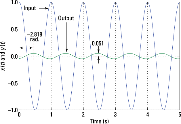
Figure 7-1: A 1-Hz sinusoid input and the corresponding steady-state sinusoid output, showing an amplitude reduction by the factor 0.051 and a phase shift by –2.818 rad.
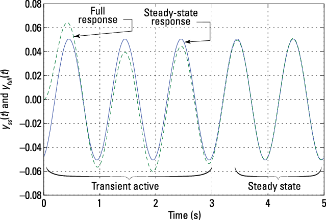
Figure 7-2: The full LCC differential equation response to a 1-Hz sinusoid, via the simulation function lsim(), overlaid with the pure steady-state portion.
Notice that the full transient solution settles to the steady-state solution in a little more than three seconds. In a real physical system, this means you can observe the steady-state response without a long wait. Good news.
Checking out the Difference Equations
Linear constant coefficient difference equations are the discrete-time cousins to the linear constant coefficient differential equations that I cover in the first half of this chapter. The convolution sum (see Chapter 6), although mathematically sound, doesn’t lend itself to practical implementation in the real world because each output y[n] may require an infinite number of calculations due to the doubly infinite sum in the definition. Fortunately, the LCC difference equation comes to the rescue, allowing for LTI systems to function on computers and all sorts of portable electronics.
For analysis purposes, solving LCC difference equations in all but the simplest cases requires more powerful mathematics than I cover in this section. Here, I limit the coverage to a general look at difference equations and the sinusoidal steady-state solution. You can further analyze LCC difference equation systems by using the frequency/Fourier domain (covered in Chapter 10) and find full time-domain solutions by using the z-transfrom (described in Chapter 13).
Modeling a system using a general Nth-order LCC difference equation
The Nth-order LCC difference equation that’s used in signals and systems, especially digital signal processing, takes the following form:
![]()
where N is the number of feedback terms (also the system order) and M is the number of feedforward terms. The coefficient sets, {ak} and {bk}, like their continuous-time counterparts, control the exact model behavior.
When you use an LCC difference equation to implement a causal LTI system, you need to rearrange it to solve for the present output, ![]() , in terms of the present input,
, in terms of the present input, ![]() , as well as past inputs and outputs. Unlike the continuous-time domain, where the model corresponds to some circuit, the difference equation in the discrete-time domain is what you implement in code! This is a very significant difference, especially given the importance discrete-time signals and systems have in today’s products.
, as well as past inputs and outputs. Unlike the continuous-time domain, where the model corresponds to some circuit, the difference equation in the discrete-time domain is what you implement in code! This is a very significant difference, especially given the importance discrete-time signals and systems have in today’s products.
Generally, ![]() ; if not, all the coefficients can be normalized by
; if not, all the coefficients can be normalized by ![]() to form the following equation:
to form the following equation:
![]()
Here, just assume that ![]() .
.
Because it involves recursion, the general LCC difference equation likely results in an impulse response of infinite duration, or an infinite impulse response (IIR) system/filter.
In Chapter 6, I introduce finite impulse response (FIR) systems. The general LCC difference equation reduces to an FIR system when ![]() and
and ![]() for
for ![]() , or
, or ![]() . Note that the convolution sum formula (see Chapter 6) with argument h[k]x[n – k] is already in the form of a feedforward-only difference equation by letting bk = h[k].
. Note that the convolution sum formula (see Chapter 6) with argument h[k]x[n – k] is already in the form of a feedforward-only difference equation by letting bk = h[k].
Example 7-2: The accumulator system has output equal to the sum of the present input and all past inputs (this system is also covered in Chapter 6). In mathematical terms, this means
![]()
You can find the impulse response for this system by setting ![]() and referring to the output as h[n]:
and referring to the output as h[n]: ![]() , which is a step function. If you’re curious what the difference equation looks like, you can find the LCC difference equation representation in two steps:
, which is a step function. If you’re curious what the difference equation looks like, you can find the LCC difference equation representation in two steps:
1. Referring to the output mathematical expression, expand the sum of all past and present inputs into two terms — the present input and a sum representing all the past inputs:
![]()
2. Observe that the sum of all past inputs (last term from Step 1) is just y[n – 1].
With this substitution, you have the nice and simple difference equation: y[n] = y[n – 1] + x[n].
Implementing the accumulator is fast and efficient because only one addition is required per output sample.
Formally, the form ![]() shows that the LCC difference equation has
shows that the LCC difference equation has ![]() with
with ![]() ,
, ![]() , and
, and ![]() with
with ![]() . Figure 7-3 shows the implementation of the accumulator system in block diagram form.
. Figure 7-3 shows the implementation of the accumulator system in block diagram form.
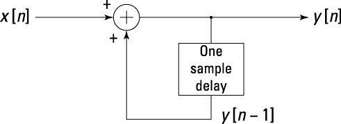
Figure 7-3: The accumulator system block diagram.
Using recursion to find the impulse response of a first-order system
Basic solution techniques exist for difference equations just as they do for differential equations, and using a recursion approach is terrific when you need to solve for only a few terms or to discover the impulse or step response of a first-order system. But when you’re solving higher-order LCC difference equations, you can do it quite efficiently with z-transform techniques (see Chapter 13) and totally avoid the use of recursion.
Using simple recursive solutions can help build confidence in working with recursive solutions and see, on a small scale, how initial conditions can be incorporated. To get started, consider the equation ![]() with initial condition
with initial condition ![]() . Using the standard LCC difference equation form, you have
. Using the standard LCC difference equation form, you have ![]() with
with ![]() , and
, and ![]() . The input
. The input ![]() is a scaled step sequence with gain K.
is a scaled step sequence with gain K.
The recursive solution just iteratively forms the output from the input and initial condition by cranking the LCC difference equation step by step, starting at ![]() .
.
To begin, take the difference equation and isolate ![]() on the left, set
on the left, set ![]() , and solve for
, and solve for ![]() :
:
![]()
For n = 1, find ![]() and so forth. You can conveniently organize the results in an equation table like this:
and so forth. You can conveniently organize the results in an equation table like this:

In this situation, a pattern develops quickly, allowing you to write a general expression for ![]() in compact form. To get to the final answer, identify and sum an embedded finite geometric series. (Flip back to Chapter 6 to see more applications of the geometric series.)
in compact form. To get to the final answer, identify and sum an embedded finite geometric series. (Flip back to Chapter 6 to see more applications of the geometric series.)
If you set ![]() and
and ![]() , the answer becomes
, the answer becomes
![]()
where s[n] denotes the step response (output of an at-rest system when x[n] = u[n]). This answer agrees exactly with the convolution sum result ![]() in Chapter 6.
in Chapter 6.
You can also find the impulse response with recursion by setting ![]() . Because the initial condition is 0 (y[–1] = 0) when finding the impulse response (see Chapter 6), the output recursion (with h[n] = y[n]) is
. Because the initial condition is 0 (y[–1] = 0) when finding the impulse response (see Chapter 6), the output recursion (with h[n] = y[n]) is ![]() , or in compact form, h[n] = an u[n].
, or in compact form, h[n] = an u[n].
The simple LCC difference equation ![]() corresponds to a system with impulse response h[n] = anu[n].
corresponds to a system with impulse response h[n] = anu[n].
Considering sinusoidal outputs in steady state
Discrete-time LTI systems, as with their continuous-time counterparts, are characterized by sinusoidal signals (sequences). This section analyzes the steady-state behavior of sinusoids in discrete-time LTI systems. The focus here is on the differences between discrete-time systems and continuous-time systems.
The general output of discrete-time LTI systems contains one or more transient terms of the form ![]() . For stable systems,
. For stable systems, ![]() , so the transient terms die out as
, so the transient terms die out as ![]() . What’s left is the steady-state response.
. What’s left is the steady-state response.
In sinusoidal steady-state analysis, you ensure that all transients decay to 0 by applying the sinusoidal input, starting from ![]() . Now when the input is a single sinusoid
. Now when the input is a single sinusoid ![]() , the steady-state output is of the form
, the steady-state output is of the form ![]() .
.
A complex sinusoid is the most useful signal for this analysis because the math is simpler, but I choose ![]() for analyses in the following sections. Note that
for analyses in the following sections. Note that ![]() is the discrete-time frequency variable and has units of rad/sample. Find details on the connection between
is the discrete-time frequency variable and has units of rad/sample. Find details on the connection between ![]() and the continuous-time frequency variables
and the continuous-time frequency variables ![]() and f in Chapters 4 and 10.
and f in Chapters 4 and 10.
Starting with a complex sinusoid
Using the convolution sum formula with x[n] representing a complex sinusoidal sequence,

The quantity, ![]() , that factors out of the convolution sum on the far right, is the discrete-time system frequency response evaluated at
, that factors out of the convolution sum on the far right, is the discrete-time system frequency response evaluated at ![]() . This is a complex quantity with polar form
. This is a complex quantity with polar form ![]() being of particular interest because the steady-state solution y[n] uses this form. The discrete-time frequency response serves the same purpose as H(f) in the continuous-time case, but it’s defined in terms of a sum rather than an integral. Another noteworthy difference is that
being of particular interest because the steady-state solution y[n] uses this form. The discrete-time frequency response serves the same purpose as H(f) in the continuous-time case, but it’s defined in terms of a sum rather than an integral. Another noteworthy difference is that ![]() is periodic with period
is periodic with period ![]() because
because
![]()
Moving on to a real sinusoid
In a development that parallels the case of the real sinusoid for continuous-time systems in the earlier section “Responding to a real sinusoid,” it can be shown that given input ![]() and a system with real impulse response h[n], the steady-state system output is
and a system with real impulse response h[n], the steady-state system output is ![]() .
.
This apparent multiplicative property, input to output holds only for sinusoids passing through LTI systems and only under steady-state conditions. For example,
![]()
This warning applies to both continuous and discrete signals and systems.
I focus on the real sinusoidal sequence input in this book because most practical systems involve real signals. You need Euler’s identity and the assumption that h[n] is real to develop the expression for y[n] in discrete- and continuous-time systems.
Solving for the general Nth-order LCC difference equation frequency response
To find the frequency response of the general LCC difference equation, first consider the complex sinusoid input/output relationship:
![]()
To develop the frequency response equation, start with the general difference equation, ![]() , and follow these steps:
, and follow these steps:
1. Make the substitution ![]() on the left and
on the left and ![]() on the right, making sure to replace n with n – k:
on the right, making sure to replace n with n – k:

2. Factor ![]() on the left side and
on the left side and ![]() on the right side.
on the right side.
The common term ![]() cancels:
cancels:
![]()
3. Solve for ![]() :
:

Unlike the continuous-time case, you develop this formula without using calculus. If you need to find the difference equation from the frequency response, just reverse the steps.
Example 7-3: Consider an M = 3 FIR filter (note N = 0 in the general LCC difference equation) with ![]() and
and ![]() . Find
. Find ![]() by using
by using ![]() . Check answers in Python.
. Check answers in Python.
Observe that ![]() . The following IPython calculations (or your calculator) can reveal that
. The following IPython calculations (or your calculator) can reveal that
![]()
In [157]: H = 1 + 2*exp(-1j*pi/5.)+3*exp(-1j*2*pi/5.)
In [158]: H
Out[158]: (3.5451-4.0287j)
In [159]: abs(H) # Magnitude at pi/5
Out[159]: 5.3664
In [160]: angle(H) # Phase at pi/5
Out[160]: -0.8491
With ![]() in hand, use the steady-state formula for the output given the input
in hand, use the steady-state formula for the output given the input ![]() :
:
