
Chapter 9
The Fourier Transform for Continuous-Time Signals and Systems
In This Chapter
![]() Checking out the world of Fourier transform for aperiodic signals
Checking out the world of Fourier transform for aperiodic signals
![]() Getting familiar with Fourier transforms in the limit
Getting familiar with Fourier transforms in the limit
![]() Working with LTI systems in the frequency domain and the frequency response
Working with LTI systems in the frequency domain and the frequency response
The Fourier transform (FT) is the gateway to the frequency domain — the “home, sweet home” of the frequency spectrum for signals and the frequency response for systems — for all your signals and systems analysis. In the time domain, the independent variable is time, t; in the frequency domain, the independent variable is frequency, f, in hertz or via a variable change ![]() in radians per second.
in radians per second.
When you take signals and systems to the frequency domain, you not only get a frequency domain view of each, but you also have the ability to perform joint math operations. The most significant is multiplication of frequency-domain quantities — the spectrum of a signal and the frequency response of a linear time-invariant (LTI) system, for example.
Consider this: The FT convolution theorem says that multiplication in the frequency domain is equivalent to convolution in the time domain. So to pass a signal through an LTI system, you just multiply the signal spectrum times the frequency response and then use the IFT to return the product to the time domain; you can totally avoid the convolution integral. Yes, there’s more where that came from in this chapter.
 The Fourier series, in general, gives you the frequency spectrum of a continuous-time periodic signal (see Chapter 8). But it has limitations. For starters, a signal has to be periodic to contain the Fourier series, which means that aperiodic signals (covered in Chapter 3) are left out of this party — until you apply the FT to remove this limitation. With regard to continuous-time signals, the FT serves most of all your spectral analysis needs. What a versatile little technique!
For discrete-time signals and systems, the FT is known as the discrete-time Fourier transform (DTFT). Check out Chapter 11 for details on the DTFT.
This chapter is devoted to frequency domain representations. (Flip to Chapter 6 if you’re looking for information on the time domain for continuous-time signals.) I describe various FT properties and theorems here and provide them in tabular form so you can access and apply them as needed in your work. I also describe filters, which is just a more descriptive name for an LTI system. Filters allow some signals to pass while blocking others.
Tapping into the Frequency Domain for Aperiodic Energy Signals
To transform a signal or system impulse response (described in Chapter 5) from the time domain to the frequency domain, you need an integral formula. Then, to get back to the time domain, you use the inverse Fourier transform (IFT), again with an integral formula.
When it comes to Fourier transforms, power and periodic go together and energy and aperiodic go together.
In this section, you begin working with the FT by exploring the amplitude and phase spectra (which are symmetry properties for real signals) and the energy spectral density. I include a collection of useful FT/IFT theorems and pairs, which makes working with the FT more efficient. Use these tables to shop for solution approaches when you’re working FT-based problems.
Working with the Fourier series
The mathematical motivation for the FT comes from the Fourier series analysis and synthesis equations for x(t) periodic that I cover in Chapter 8. To visualize the Fourier transform, consider the pulse train signal (described in Chapter 8) with pulse width ![]() fixed. When you let the period T0 grow to infinity, the pulse train becomes an isolated pulse, an aperiodic signal. Figure 9-1 shows side-by-side plots of the pulse train waveform x(t) and the normalized amplitude line spectra as T0 is stepped over
fixed. When you let the period T0 grow to infinity, the pulse train becomes an isolated pulse, an aperiodic signal. Figure 9-1 shows side-by-side plots of the pulse train waveform x(t) and the normalized amplitude line spectra as T0 is stepped over ![]() and then to infinity. (I plot
and then to infinity. (I plot ![]() to maintain a constant spectral height as T0 changes.)
to maintain a constant spectral height as T0 changes.)
The spectral lines get closer together as T0 increases because the line spacing is the fundamental frequency f0 = 1/T0. In the last row, T0 goes to infinity, which makes x(t) a single rectangular pulse and the line spectrum a continuous function of frequency f. This solution reveals the Fourier transform of the ![]() -width rectangular pulse, which you find by using the Fourier transform in the next section, Example 9-1.
-width rectangular pulse, which you find by using the Fourier transform in the next section, Example 9-1.
In Figure 9-1, the pulse train has Fourier coefficient magnitude ![]() , where
, where ![]() . To maintain a constant spectral height in the plots, I normalize Xn as
. To maintain a constant spectral height in the plots, I normalize Xn as ![]() .
.
The line spectra is really just sampling the function ![]() at f = nf0. When
at f = nf0. When ![]() , you also have
, you also have ![]() and can let
and can let ![]() such that
such that ![]() . This limiting argument makes
. This limiting argument makes ![]() , which is the FT of the aperiodic signal
, which is the FT of the aperiodic signal ![]() .
.
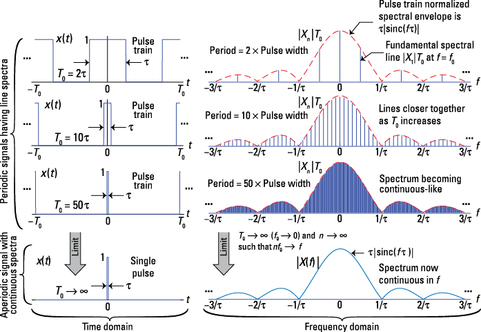
Figure 9-1: Morphing a pulse train, viewed in the time and frequency domains, into a single pulse by letting T0 approach infinity while holding the pulse width ![]() fixed.
fixed.
Using the Fourier transform and its inverse
To get to the FT, x(t) must be aperiodic — and have finite energy (energy signals are covered in Chapter 3): ![]() .
.
The forward FT is given by ![]() , with
, with ![]() being the frequency domain representation of
being the frequency domain representation of ![]() . By formalizing the limit arguments described in the previous section, you can return to the time domain by using the inverse Fourier transform (IFT):
. By formalizing the limit arguments described in the previous section, you can return to the time domain by using the inverse Fourier transform (IFT):
![]()
Using the calligraphy character ![]() to denote the FT and
to denote the FT and ![]() to denote the IFT is common practice because it’s clearly distinguishable. For instance, F{x(t)} may represent some function of x(t) but not necessarily the Fourier transform. This practice reserves the roman F to be safely used for other purposes.
to denote the IFT is common practice because it’s clearly distinguishable. For instance, F{x(t)} may represent some function of x(t) but not necessarily the Fourier transform. This practice reserves the roman F to be safely used for other purposes.
The transform ![]() is known as the spectrum of
is known as the spectrum of ![]() and is a continuous function of frequency. In general, it’s also complex. Here are a couple of things to know about units associated with X(f):
and is a continuous function of frequency. In general, it’s also complex. Here are a couple of things to know about units associated with X(f):
![]() If
If ![]() has units of voltage, then
has units of voltage, then ![]() has units v-s or v/Hz, because time and frequency are reciprocals.
has units v-s or v/Hz, because time and frequency are reciprocals.
![]() The IFT faithfully returns
The IFT faithfully returns ![]() to the time domain and the original units of volts.
to the time domain and the original units of volts.
 You can also apply the Fourier transform to signals by using a radian frequency variable
 ![]() . The forward and inverse transforms in this case are
. The forward and inverse transforms in this case are
![]()
In this book, I use the frequency variable f, which has units of hertz, and the corresponding FT/IFT integral formulas presented at the beginning of this section. Other books may use the radian frequency variable. The tables of transform theorems and transform pairs in this chapter (see Figures 9-3 and 9-9) contain an extra column for ![]() to make it easier for you to adapt this info to your specific needs.
to make it easier for you to adapt this info to your specific needs.
 Example 9-1: Consider this pulse signal:
![]()
Use the definition of the FT, the integral formula, that takes you from the time domain, x(t), to the frequency domain, X(f):

In the third line, I use Euler’s formula for sine. To get to the last line, I use the function ![]() (defined in Chapter 8).
(defined in Chapter 8).
The sinc function is quite popular when dealing with Fourier transforms. Whenever rectangular pulse functions are present in the time domain, you find a sinc function in the frequency domain. Knowing sinc spectral shapes comes in handy when you’re working with digital logic and communication waveforms. Check out a plot of the sinc function in Figure 9-2.
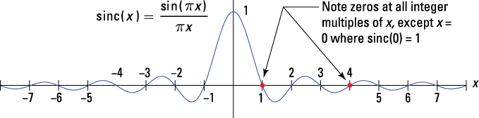
Figure 9-2: A plot of the sinc function.
The sinc function has periodic zeros at the integers ![]() and so on. By using L’Hôspital’s rule, you find out that sinc(0) = 1:
and so on. By using L’Hôspital’s rule, you find out that sinc(0) = 1:
![]()
In this example, the first spectral null occurs when ![]() or
or ![]() Hz, establishing the important Fourier transform pair:
Hz, establishing the important Fourier transform pair:
![]()
You can denote FT pairs with the double arrow ![]() .
.
Oh, I almost forgot; beyond the sinc function is the term ![]() , which occurs due to the time shift of the rectangular pulse. If
, which occurs due to the time shift of the rectangular pulse. If ![]() , this term goes away. It contributes only to the angle of
, this term goes away. It contributes only to the angle of ![]() .
.
Example 9-2: Consider this aperiodic signal:
![]()
The following steps show you how to sketch ![]() for
for ![]() and find its FT:
and find its FT:
1. Add the two piecewise continuous pulse functions, accounting for the fact that the ![]() -width pulse fits inside the
-width pulse fits inside the ![]() -width pulse.
-width pulse.
Using the definition of ![]() established in Example 9-1, you get this:
established in Example 9-1, you get this:

See the corresponding sketch in Figure 9-3.

Figure 9-3: Waveform plot of ![]() .
.
2. Find ![]() by plugging x(t) into the definition. Then form two integrals:
by plugging x(t) into the definition. Then form two integrals:

3. Recognize that each FT integral in the second line of Step 2 is a sinc function.
When you plug in the problem-specific constants, you get this equation:
![]()
This example demonstrates that the FT is a linear operator:
![]()
Getting amplitude and phase spectra
The very nature of the FT, the integral definition, makes X(f) a complex valued function of frequency f. As with any complex valued function, you can consider the rectangular form’s real and imaginary parts or the polar form’s magnitude and angle.
The polar form is the most common way of characterizing X(f). The magnitude |X(f)| is known in some circles as the amplitude spectrum; others prefer the more mathematically precise term magnitude spectrum. I use these two terms interchangeably. The angle ![]() is called the phase spectrum.
is called the phase spectrum.
![]()
Amplitude and phase spectra also exist for periodic signals in the form of line spectra (see Chapter 8). Refer to Figure 9-1 to see how the spectral representations for these two signal classifications are related.
Seeing the symmetry properties for real signals
For the case of ![]() , a real valued signal (imaginary part zero), some useful properties hold:
, a real valued signal (imaginary part zero), some useful properties hold:
![]() With Euler’s identity, you can expand the complex exponential in the FT integral as
With Euler’s identity, you can expand the complex exponential in the FT integral as ![]() . Then just calculate the real and imaginary parts of
. Then just calculate the real and imaginary parts of ![]() by using this expansion inside the FT integral:
by using this expansion inside the FT integral:

![]() Because cosine is an even function,
Because cosine is an even function, ![]() , and sine is an odd function,
, and sine is an odd function, ![]() ,
, ![]() is related to
is related to ![]() , as shown in this equation:
, as shown in this equation:

You can conclude that ![]() is conjugate symmetric, which means that its function conjugated (sign changed on the imaginary part with no change to the real part) on the positive axis and mirrors the corresponding function on the negative axis:
is conjugate symmetric, which means that its function conjugated (sign changed on the imaginary part with no change to the real part) on the positive axis and mirrors the corresponding function on the negative axis: ![]() .
.
![]() Conjugate symmetry reveals that
Conjugate symmetry reveals that
![]()
Example 9-3: Based on the results of Example 9-1, a rectangular pulse of amplitude A, pulse width ![]() , and time shift t0 has FT
, and time shift t0 has FT ![]() . Let A = 1,
. Let A = 1, ![]() and plot the amplitude and phase spectra for
and plot the amplitude and phase spectra for ![]() Hz. Plugging values into the general result of Example 9-1, the functions are the last two lines of the following equation:
Hz. Plugging values into the general result of Example 9-1, the functions are the last two lines of the following equation:

Although real, ![]() has an associated angle; negative values imply a
has an associated angle; negative values imply a ![]() radians phase shift.
radians phase shift.
You can create the plot with Python and Pylab and take advantage of the abs() and angle() functions to do the heavy lifting for this problem. Here are the essential commands:
In [132]: f = arange(-3,3,.01)
In [133]: X = 2*sinc(2*f)*exp(-1j*2*pi*f/3)
In [136]: plot(f,abs(X))
In [138]: plot(f,angle(X))
The two plots that this code creates are shown in Figure 9-4.
The amplitude plot in Figure 9-4 follows from the earlier plot of the sinc function in Figure 9-2. The magnitude operation flips the sinc function’s negative dips to the top side of the frequency axis, making a series of side lobes on both sides of the main lobe that’s centered at f = 0. The main lobe extends along the frequency axis from –1/2 to 1/2 Hz because ![]() is the location of the first spectral null, or 0, as f increases from 0 Hz.
is the location of the first spectral null, or 0, as f increases from 0 Hz.
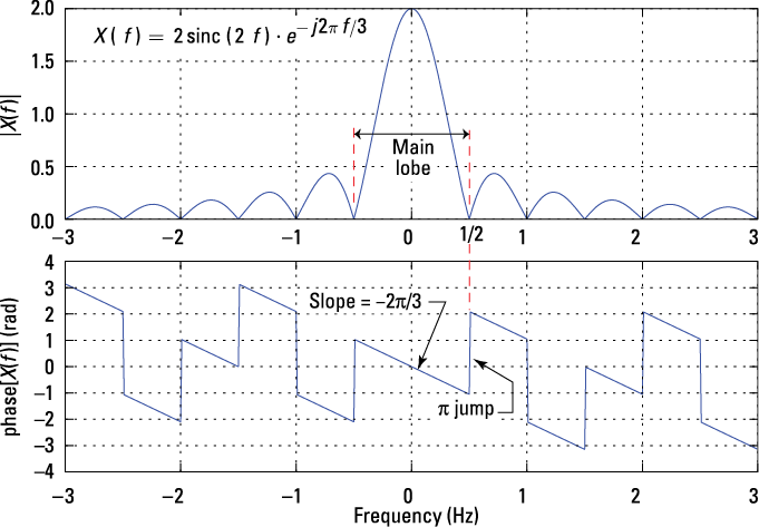
Figure 9-4: The amplitude and phase spectra of a single rectangular pulse ![]()
![]() .
.
In the phase plot, the angle of the product of two complex numbers is the sum of the angles (find a review of complex arithmetic in Chapter 2). The phase of the first term, the sinc function, comes from sign changes only, so it contributes an angle (phase) of 0 or π. The second term is in polar form already, so the phase is simply ![]() , which is a phase slope of
, which is a phase slope of ![]() . Combining terms, you get the steady phase slope with phase jumps by
. Combining terms, you get the steady phase slope with phase jumps by ![]() being interjected whenever the sinc function is negative, creating a scenario in which the phase plot jumps up and down at integer multiples of
being interjected whenever the sinc function is negative, creating a scenario in which the phase plot jumps up and down at integer multiples of ![]() .
.
In general, a phase plot includes only the principle values ![]() . When the phase attempts to go below –π or above π, the
. When the phase attempts to go below –π or above π, the angle() function in PyLab wraps the phase modulo ![]() by either adding or subtracting
by either adding or subtracting ![]() , and this explains why phase plots can have
, and this explains why phase plots can have ![]() and
and ![]() jumps. You can find the unwrapped phase by using the function
jumps. You can find the unwrapped phase by using the function unwrap(angle()).
Figure 9-4 also shows that the amplitude spectrum is even and the phase spectrum is odd for real ![]() . Two additional properties pertain to even and odd symmetry of
. Two additional properties pertain to even and odd symmetry of ![]() . The function go(t) is odd if go(–t) = –go(t). When you integrate this function over symmetrical limits, you get 0. To verify this, follow these two steps:
. The function go(t) is odd if go(–t) = –go(t). When you integrate this function over symmetrical limits, you get 0. To verify this, follow these two steps:
1. Integrate go(t) with symmetrical limits [–L, L] by breaking the integral into the interval [–L, 0] and [0, L]:
![]()
2. Change variables in the first integral by letting u = –t, which also means –dt = du and the limits now run over [L, 0].
With a sign change to the first integral, you can change the limits to match the first integral:
![]()
The even and odd symmetry properties reveal these solutions:
![]() For
For ![]() even, or
even, or ![]() ,
,
![]()
![]() For
For ![]() odd,
odd, ![]() ,
,
![]()
Refer to ![]() , Example 9-2, and Figure 9-3. The imaginary part of
, Example 9-2, and Figure 9-3. The imaginary part of ![]() must be 0 because
must be 0 because ![]() is even. Look at the solution for
is even. Look at the solution for ![]() in Example 9-2. It’s true! The sum of two sinc functions is a real spectrum.
in Example 9-2. It’s true! The sum of two sinc functions is a real spectrum.
Example 9-4: Consider the signal ![]() shown in Figure 9-5.
shown in Figure 9-5.
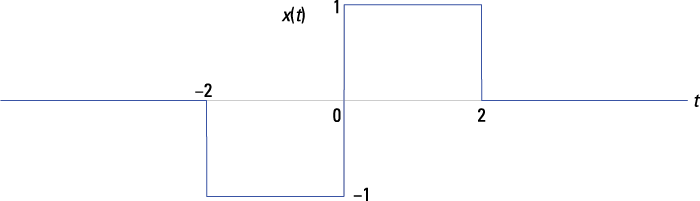
Figure 9-5: The difference of two rectangular pulses configured to create an odd function.
In mathematical terms, x(t) can be written as the difference between two time-shifted rectangular pulse functions: ![]() .
.
Find the FT of ![]() by using the FT linearity property described in Example 9-2. Because
by using the FT linearity property described in Example 9-2. Because ![]() ,
,

In the last line, I use Euler’s inverse formula for sine to simplify the expression for X(f).
In Figure 9-5, ![]() has odd symmetry, so you may assume that
has odd symmetry, so you may assume that ![]() is pure imaginary or real part identically 0. You’re right; it is!
is pure imaginary or real part identically 0. You’re right; it is!
Finding energy spectral density with Parseval’s theorem
The energy spectral density of energy signal ![]() is defined as
is defined as ![]() . The units of X(f) are v-s (covered in the section “Using the Fourier transform and its inverse,” earlier in this chapter), so squaring in a 1-ohm system reveals that W-s2 = W-s/Hz = Joules/Hz. Indeed, the units correspond to energy per hertz of bandwidth.
. The units of X(f) are v-s (covered in the section “Using the Fourier transform and its inverse,” earlier in this chapter), so squaring in a 1-ohm system reveals that W-s2 = W-s/Hz = Joules/Hz. Indeed, the units correspond to energy per hertz of bandwidth.
In Chapter 8, I describe Parseval’s theorem for power signals; here’s how the theorem applies to energy signals:
![]()
Use this theorem to integrate the energy spectral density of a signal over all frequency to get the total signal energy.
Getting the proof for Parseval’s theorem
The proof for Parseval’s theorem is straightforward. Two steps, and you’re done:
1. Start from the time-domain side of the theorem by writing the integrand as ![]() , and then replace x(t) with the IFT integral formula:
, and then replace x(t) with the IFT integral formula:
![]()
2. Rewrite the results of Step 1 by interchanging the integration order and recognizing that the inner integral involving ![]() is just the conjugate of X(f).
is just the conjugate of X(f).
You’re left with ![]() as the integrand of the remaining integral:
as the integrand of the remaining integral:
![]()
Example 9-5: Find the signal energy and sketch the energy spectral density in decibels (dB) for the signals ![]() (a rectangle pulse) and
(a rectangle pulse) and ![]() (a bi-phase pulse).
(a bi-phase pulse).
The spectrum of x1(t) is ![]() with
with ![]() , and X2(f) is identical to the results of Example 9-5. Both signals have a total pulse width of 4 s. To fairly compare the energy spectral densities, you need each of the pulses to have the same total energy. Using the time-domain version of Parseval’s theorem (covered in Chapter 3), you find the signal energy by integrating |x(t)|2 over the pulse duration:
, and X2(f) is identical to the results of Example 9-5. Both signals have a total pulse width of 4 s. To fairly compare the energy spectral densities, you need each of the pulses to have the same total energy. Using the time-domain version of Parseval’s theorem (covered in Chapter 3), you find the signal energy by integrating |x(t)|2 over the pulse duration:

Good, the energies are equal. To plot the energy spectral density in dB means that you plot ten times the base ten log of the energy spectrum. The energy spectral densities you plot are

If you want to plot the energy spectral density in dB using Python and PyLab, use these essential commands:
In [179]: f = arange(-2,2,.01)
In [180]: X1 = abs(4*sinc(4*f))**2
In [181]: X2 = abs(4*sinc(2*f)*sin(2*pi*f))**2
In [181]: plot(f,10*log10(X1))
In [182]: plot(f,10*log10(X2))
Check out the results in Figure 9-6.
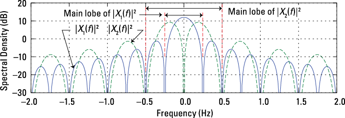
Figure 9-6: Energy spectral density in dB comparison for 4-s rectangle and bi-phase pulses.
In communications and radar applications, the energy spectral density is an important design characteristic. The rectangular and bi-phase pulse shapes used here are popular in wired digital communications. The main lobe for each of the energy spectral densities is noted in Figure 9-6. The main lobe serves as a measure of spectral bandwidth. I can define the signal bandwidth B as the frequency span from 0 Hz to the location of the first spectral null, the point where the spectrum is 0 or negative infinity in dB. The first null of the rectangle pulse spectrum is one over the pulse width or B1 = 0.25 Hz. For the bi-phase pulse, the bandwidth is B2 = 0.5 Hz. The rectangle pulse seems like the bandwidth-efficient choice, but the bi-phase pulse doesn’t contain any spectral energy at direct current (DC; f = 0), which means it can pass through cable interfaces that block DC.
Applying Fourier transform theorems
A handful of the most popular FT theorems can make life so much more pleasant. I summarize helpful theorems in Figure 9-7 and describe the core theorems in this section. The featured theorems are applicable in many electrical engineering situations. Other theorems have special application, and having them handy when they’re needed is mighty nice.
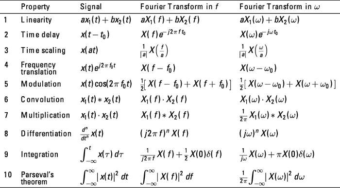
Figure 9-7: Fourier transform theorems.
Linearity
The linearity theorem tells you that a linear combination of signals can be transformed term by term:
![]()
The proof of this theorem follows from the linearity of integration itself:
![]()
I use this theorem for the solution of Example 9-2.
Time delay
The time delay theorem tells you how the FT of a time-delayed signal is related to the FT of the corresponding undelayed signal. I cover time-shifting signals in Chapter 3; here you can see what this technique looks like in the frequency domain.
![]()
 Here’s the proof. I use the variable substitution
 ![]() , which results in
, which results in ![]() and
and ![]() , followed by a factoring of
, followed by a factoring of ![]() :
:

I put the time delay theorem in action in Example 9-1 to find ![]() It’s important to remember that
It’s important to remember that ![]() . With the t replaced by t – t0, you modify the FT by simply including the extra term
. With the t replaced by t – t0, you modify the FT by simply including the extra term ![]() .
.
Frequency translation
The frequency translation theorem can help you find the frequency-domain impact of multiplying a signal by a complex sinusoid ![]() . The theorem tells you that the spectrum of x(t) is shifted up in frequency by f0.
. The theorem tells you that the spectrum of x(t) is shifted up in frequency by f0.
In communication applications, frequency translation is a common occurrence; after all, translating a signal from one frequency location to another is how signals are transmitted and received wirelessly. This theorem is also the foundation of the modulation theorem.
![]()
To prove, combine the exponential terms in the FT integral and then notice that the new frequency variable for the FT integral is ![]() — just x(t) being transformed:
— just x(t) being transformed:
![]()
Example 9-6: An extremely practical application of the frequency translation theorem is finding the FT of ![]() . The first step is to expand the cosine by using Euler’s formula:
. The first step is to expand the cosine by using Euler’s formula:
![]()
Then apply the linearity theorem to the expanded form:

With that, you established the modulation theorem. Read on for details.
Modulation
The modulation theorem is similar to the frequency translation theorem; only now a real sinusoid ![]() replaces the complex sinusoid. This shifts the spectrum of x(t) up and down in frequency by f0.
replaces the complex sinusoid. This shifts the spectrum of x(t) up and down in frequency by f0.
![]()
Example 9-7: The block diagram of Figure 9-8 is a simple modulator that places the signal x(t) on the carrier frequency f0.
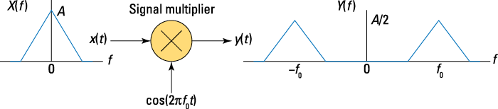
Figure 9-8: A simple modulator that forms ![]()
![]() .
.
The only system building block required for this example is the ideal multiplier, which forms y(t) as the product of x(t) and ![]() . Notice that y(t) fits the modulation theorem perfectly. The modulation theorem says
. Notice that y(t) fits the modulation theorem perfectly. The modulation theorem says ![]() .
.
The input spectrum X(f) is centered at f = 0 with peak spectrum amplitude A. The output spectrum sketch Y(f) in Figure 9-6 reveals that multiplication by ![]() has shifted the input spectrum X(f) up and down in frequency by f0 Hz and scaled the spectral amplitude by 1/2. By translating the input spectrum up and down in frequency, you place the information conveyed by x(t) at a frequency that allows for easy wireless transmission. At the receiver, a demodulator recovers x(t) from y(t).
has shifted the input spectrum X(f) up and down in frequency by f0 Hz and scaled the spectral amplitude by 1/2. By translating the input spectrum up and down in frequency, you place the information conveyed by x(t) at a frequency that allows for easy wireless transmission. At the receiver, a demodulator recovers x(t) from y(t).
Duality
The duality theorem tells you that role reversal is possible with the FT. Literally, it just means that x(t) is taken as X(t), and X(f) is taken as x(–f). The theorem statement is ![]() .
.
In words, the Fourier transform of a spectrum X(f), with f replaced by t, is time-domain quantity x(t) with t replaced by –f. The time delay and frequency translation theorems described earlier in this section demonstrate this behavior.
![]() The time delay theorem states that a delay in the time domain means multiplication by a complex exponential in the frequency domain.
The time delay theorem states that a delay in the time domain means multiplication by a complex exponential in the frequency domain.
![]() Duality says a frequency shift in the frequency domain should result in multiplication by a complex exponential in the time domain.
Duality says a frequency shift in the frequency domain should result in multiplication by a complex exponential in the time domain.
Hey! That’s exactly what the frequency translation theorem does.
Example 9-8: A great application of the duality theorem is in finding the IFT of the rectangular spectrum ![]() . The first step is to insert X(f) in the left side of the theorem with f replaced by t:
. The first step is to insert X(f) in the left side of the theorem with f replaced by t: ![]() . The second step is to find the FT of X(t).
. The second step is to find the FT of X(t).
Because ![]() , the theorem tells you that the right side is x(–f), so
, the theorem tells you that the right side is x(–f), so ![]() . The little detail of x(–f) = x(f) follows from the sinc function being even.
. The little detail of x(–f) = x(f) follows from the sinc function being even.
In the final step, swap variables back: ![]() . A handy transform pair emerges — without doing any integration:
. A handy transform pair emerges — without doing any integration:
![]()
Proving duality
To prove the duality theorem, use direct substitution into the FT definition:
![]()
In the last step, the integral is viewed as the IFT with the variable of integration role reversed. In other words, t takes the place of f in the IFT, and then you identify the independent variable as –f.
You can now say that as a result of duality, a sinc in the time domain is a rectangle in the frequency domain. Add this one to your toolbox!
Convolution
The convolution theorem is worthy of a drum roll. Yes, it’s that special. The convolution theorem is one of the most powerful FT theorems, and it’s especially useful in communications applications.
The convolution theorem considers ![]() in terms of the FT, where it can be shown that
in terms of the FT, where it can be shown that ![]() . This result is significant because it tells you that convolution in the time domain becomes simple multiplication in the frequency domain. I’m guessing that you may be falling in love with convolution integrals right now.
. This result is significant because it tells you that convolution in the time domain becomes simple multiplication in the frequency domain. I’m guessing that you may be falling in love with convolution integrals right now.
Note that x2(t) may also be an LTI system impulse response, making ![]() the output if x1(t) is the input. This aspect of the convolution theorem is explored in the later section “LTI Systems in the Frequency Domain.”
the output if x1(t) is the input. This aspect of the convolution theorem is explored in the later section “LTI Systems in the Frequency Domain.”
The proof involves direct application of the IFT and FT definitions and interchanging orders of integration:

Example 9-9: Find the FT of ![]() , using the convolution theorem
, using the convolution theorem ![]() .
.
In Chapter 5, I point out that the convolution of two signals is defined as ![]() . Because convolving two equal-width rectangles yields a triangle, and the height of the triangle is the area of the full overlap,
. Because convolving two equal-width rectangles yields a triangle, and the height of the triangle is the area of the full overlap,
![]()
Putting the two sides together and removing a ![]() for each side establishes the FT pair:
for each side establishes the FT pair:
![]()
Multiplication
The multiplication theorem is the convolution theorem times two; this one considers the FT as the product of two signals. In communication systems and signal processing, this theorem is quite useful.
Whereas the modulation theorem involved a signal multiplied by a cosine, the multiplication theorem is a generalization because both signals are arbitrary.
Based on the convolution and duality theorems described earlier in this section, it follows that ![]() .
.
Example 9-10: If ![]() , find
, find ![]() . Start by finding
. Start by finding ![]() . Example 9-8 established the FT pair
. Example 9-8 established the FT pair ![]() . Here, 2W = 3 and thus
. Here, 2W = 3 and thus ![]() . So you can convolve identical rectangle shapes to get the triangle
. So you can convolve identical rectangle shapes to get the triangle ![]() .
.
An alternative approach to this problem is to use the dual of the transform pair ![]() established in Example 9-9. Try this approach on your own.
established in Example 9-9. Try this approach on your own.
Checking out transform pairs
A pair is simply the corresponding time- and frequency-domain function that emerges from a FT/IFT combination. And after you develop the FT pair for a particular signal, you can use it over and over again as you work problems.
Figure 9-9 shows the most popular FT pairs — some of which rely on the Fourier transform in the limit concept. Several of these pairs are developed in the examples in this section.
Example 9-11: Develop the FT pair for ![]() , which corresponds to Figure 9-9 Line 7:
, which corresponds to Figure 9-9 Line 7:
![]()
The dual version of this pair is Figure 9-9 Line 8, ![]() , which is actually a Fourier transform in the limit result.
, which is actually a Fourier transform in the limit result.
The reciprocal spreading property of pulse signals and their corresponding spectra states that a signal with a wide pulse has a narrow spectrum while a signal with a narrow pulse has a wide spectrum. So, roughly speaking, the time spread and frequency spread of a pulse signal and its spectrum are reciprocals.
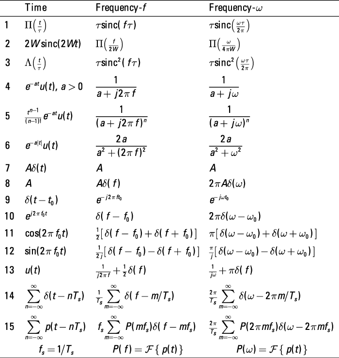
Figure 9-9: Fourier transform pairs; those containing an impulse function in the frequency domain are transforms in the limit.
Consider the impulse signal and the constant signals, whose Fourier transforms are found in Figure 9-9 Lines 7 and 8. For the impulse signal, one over the time duration yields a signal bandwidth of infinity; and for the constant signal, one over the signal duration of infinity yields a signal bandwidth of zero.
A more typical scenario is the rectangle pulse of duration ![]() s (Figure 9-9 Line 1). This signal has a sinc function spectrum, where the main spectral lobe has single-sided width
s (Figure 9-9 Line 1). This signal has a sinc function spectrum, where the main spectral lobe has single-sided width ![]() Hz (refer to Figure 9-4). Reciprocal spreading applies here.
Hz (refer to Figure 9-4). Reciprocal spreading applies here.
Getting Around the Rules with Fourier Transforms in the Limit
Formally, the Fourier transform (FT) requires ![]() to be an energy signal. But you don’t need to always be so picky. In this section, I show you how to find the FT of power signals, including sine/cosine and periodic pulse signals, such as the pulse train. The technique is known as Fourier transforms in the limit, and it allows you to bring together spectral analysis of both power and energy signals in one frequency-domain representation, namely X(f). The trick is getting singularity functions, particularly the impulse function, into the frequency domain.
to be an energy signal. But you don’t need to always be so picky. In this section, I show you how to find the FT of power signals, including sine/cosine and periodic pulse signals, such as the pulse train. The technique is known as Fourier transforms in the limit, and it allows you to bring together spectral analysis of both power and energy signals in one frequency-domain representation, namely X(f). The trick is getting singularity functions, particularly the impulse function, into the frequency domain.
Using the Fourier transform in the limit, I show you how to find the FT of any periodic power signal. This leads to unifying the spectral view of both periodic power signals and aperiodic energy signals under the Fourier transform.
Handling singularity functions
Singularity functions include the impulse function and the step function. Getting the impulse function into the frequency domain is a great place to start working with the Fourier transform in the limit.
Consider a constant signal ![]() . You can write this signal in limit form:
. You can write this signal in limit form:
![]() , where
, where ![]()
The Fourier transform in the limit of ![]() is
is ![]() . Figure 9-10 shows what happens as T increases to
. Figure 9-10 shows what happens as T increases to ![]() .
.
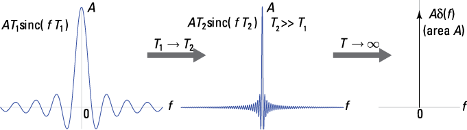
Figure 9-10: The result of increasing T in ![]()
![]() .
.
Because ![]() is a constant and has no time variation, the spectral content of
is a constant and has no time variation, the spectral content of ![]() ought to be confined to
ought to be confined to ![]() . It can also be shown that
. It can also be shown that ![]() .
.
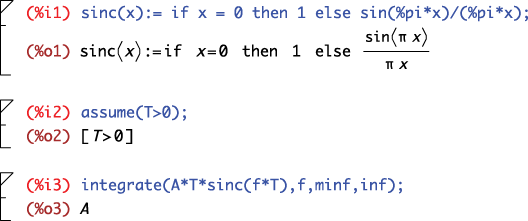
A quick symbolic integration check in Maxima confirms this.
Refer to the Fourier transform in the limit conclusion on the right side of Figure 9-7: ![]() . As a further check, consider the inverse Fourier transform (IFT)
. As a further check, consider the inverse Fourier transform (IFT) ![]() . Smooth sailing back to the time domain. Find more Fourier transform in the limit examples in Figure 9-9.
. Smooth sailing back to the time domain. Find more Fourier transform in the limit examples in Figure 9-9.
Unifying the spectral view with periodic signals
A periodic signal having period ![]() —
— ![]() — has this complex exponential Fourier series representation:
— has this complex exponential Fourier series representation:
![]()
Get the Fourier coefficients by using the formula ![]() .
.
Line 1 of Figure 9-7 and Line 10 of Figure 9-9 can help you find the FT:

For this solution to be useful, you need the Fourier series coefficients ![]() .
.
This result shows that the spectrum of a periodic signal ![]() consists of spectral lines located at frequencies
consists of spectral lines located at frequencies ![]() along the frequency axis via impulse functions. The spectral representation with terms
along the frequency axis via impulse functions. The spectral representation with terms ![]() resembles the line spectra in Chapter 8; in this chapter, you use impulse functions to actually locate the spectral lines.
resembles the line spectra in Chapter 8; in this chapter, you use impulse functions to actually locate the spectral lines.
The best thing about this FT is that it brings both aperiodic and periodic signals into a common spectral representation.
Example 9-12: Consider the ideal sampling waveform:
![]()
The Fourier series coefficients of this periodic signal are ![]() for any n. Note that
for any n. Note that ![]() is the sampling rate. With the Fourier series coefficients known, from this FT,
is the sampling rate. With the Fourier series coefficients known, from this FT, ![]() .
.
You’ve just established the FT pair of Figure 9-9 Line 14:
![]()
This FT pair is special because the signal and transform have the same mathematical form!
Two other signals have this same property; they’re the zero signal and the Gaussian shaped pulse pair.
Wouldn’t it be nice if you could find the FT of a periodic signal ![]() without having to first find the Fourier series coefficients? Well, you can! Simply start with an alternative representation of
without having to first find the Fourier series coefficients? Well, you can! Simply start with an alternative representation of ![]() , such as the following, where
, such as the following, where ![]() represents one period of
represents one period of ![]() :
:
![]()
The following FT pair (Figure 9-9 Line 15) does the trick:
![]()
Note that ![]() and
and ![]() . Figure 9-11 shows this FT pair.
. Figure 9-11 shows this FT pair.
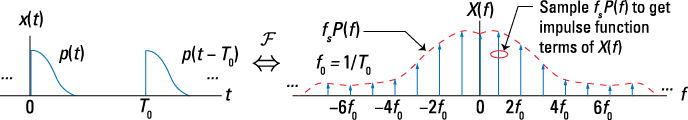
Figure 9-11: Finding the FT of a periodic sequence by sampling the spectrum P(f) of one period of x(t) at f = n/T0
From the convolution theorem (Figure 9-7 Line 6),

Example 9-13: Find the spectrum of the periodic pulse train signal ![]() . Because
. Because ![]() , Figure 9-9 Line 1 and Figure 9-7 Line 2 shows that
, Figure 9-9 Line 1 and Figure 9-7 Line 2 shows that ![]() . Using the Figure 9-9 Line 15 result, you find the following:
. Using the Figure 9-9 Line 15 result, you find the following:
![]()
A little secret: Because the form is equivalent to using the Fourier series coefficients, you can assume that the coefficients are ![]() and so on. Not a single integration required!
and so on. Not a single integration required!
LTI Systems in the Frequency Domain
Chapter 5 establishes time-domain relationships for signals interacting with LTI systems. In this section, I present the corresponding frequency-domain results for signals interacting with LTI systems, beginning with the frequency response of an LTI system in relation to the convolution theorem. I introduce you to properties of the frequency response and present a case study with an RC low-pass filter that’s connected with the linear constant coefficient (LCC) differential equation representation of LTI systems (see Chapter 7).
But don’t worry; I also touch on cascade and parallel connection of LTI systems, or filters, in the frequency domain. Ideal filters are good for conceptualizing design, but they can’t be physically realized. Realizable filters can be built but aren’t as mathematically pristine as ideal filters.
Checking out the frequency response
For LTI systems in the time domain, a fundamental result is that the output ![]() is the input
is the input ![]() convolved with the system impulse response
convolved with the system impulse response ![]() :
:![]() . In the frequency domain, you can jump right into this expression by taking the Fourier transform (FT) of both sides:
. In the frequency domain, you can jump right into this expression by taking the Fourier transform (FT) of both sides: ![]() .
.
The quantity ![]() is known as the frequency response, or transfer function, of the system having impulse response
is known as the frequency response, or transfer function, of the system having impulse response ![]() . This is a special FT because H(f) is the frequency response, not the spectrum of a signal.
. This is a special FT because H(f) is the frequency response, not the spectrum of a signal.
In Chapter 7, I hone in on the frequency response for systems described by LCC differential equations, using the sinusoidal steady-state response. This is the same frequency response I’m describing in this chapter, but now you get it as the FT of the system impulse response. This convergence of theories shows you that you can arrive at a frequency response in different ways.
If you want to find ![]() via multiplication in the frequency domain, you just need to use the inverse Fourier transform (IFT):
via multiplication in the frequency domain, you just need to use the inverse Fourier transform (IFT): ![]() .
.
Solving for H(f) in the expression for Y(f), ![]() , shows you the ratio of the output spectrum over the input spectrum. So if
, shows you the ratio of the output spectrum over the input spectrum. So if ![]() , then
, then ![]() and the output spectrum takes its shape entirely from
and the output spectrum takes its shape entirely from ![]() because
because ![]() .
.
Evaluating properties of the frequency response
For ![]() real, it follows that
real, it follows that ![]() (see the section “Seeing the symmetry properties for real signals,” earlier in this chapter). The output energy spectral density is related to the input energy spectral density and the frequency response:
(see the section “Seeing the symmetry properties for real signals,” earlier in this chapter). The output energy spectral density is related to the input energy spectral density and the frequency response: ![]() .
.
Example 9-14: Consider the RC low-pass filter circuit shown in Figure 9-12.
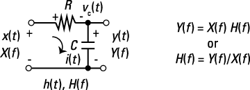
Figure 9-12: RC low-pass filter circuit and frequency-domain relationships.
To find ![]() , you can use AC steady-state circuit analysis, the Fourier transform of the impulse response, or apply the Fourier transform for the circuit differential equation term by term and solve for H(f). The impulse response is derived for this circuit in Chapter 7, so I use this same approach here:
, you can use AC steady-state circuit analysis, the Fourier transform of the impulse response, or apply the Fourier transform for the circuit differential equation term by term and solve for H(f). The impulse response is derived for this circuit in Chapter 7, so I use this same approach here:
![]()
Apply the Fourier transform to h(t), using Figure 9-9 Line 4 along with linearity:

Here, ![]() is known as the filter 3-dB cutoff frequency because
is known as the filter 3-dB cutoff frequency because
![]() .
.
Figure 9-13 illustrates the frequency response magnitude and phase and reveals the spectral shaping offered by the RC low-pass filter. The output spectrum is Y(f) = X(f)H(f), so you can deduce that signals with spectral content less than f3 are nominally passed (![]() ) while spectral content greater than f3 is attenuated, because |H(f)| shrinks to 0 as f increases (
) while spectral content greater than f3 is attenuated, because |H(f)| shrinks to 0 as f increases (![]() ).
).
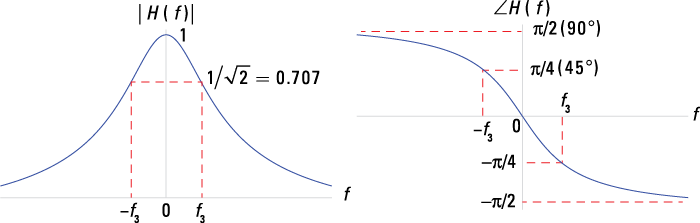
Figure 9-13: RC low-pass filter frequency response in terms of magnitude and phase plots.
Formally, a low-pass filter passes spectral content from 0 to B Hz and blocks spectral content above B Hz. Here, B is equivalent to the 3-dB frequency f3. More detail on filters is coming up later in this chapter.
Getting connected with cascade and parallel systems
As a result of the FT convolution theorem, the cascade and parallel connections in the frequency domain have an equivalent function to those in the time domain. You can develop the corresponding relationships from the block diagram in Figure 9-14.
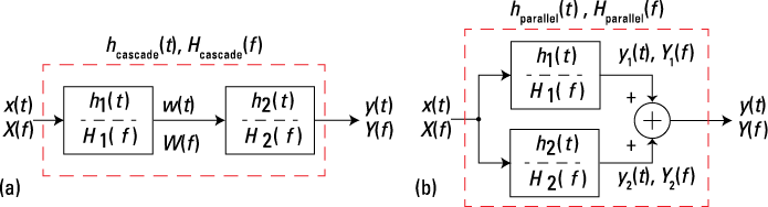
Figure 9-14: Cascade (a) and parallel (b) connected LTI systems in the frequency domain.
For the cascade system connection in the frequency domain, W(f) = X(f)H1(f) and Y(f) = W(f)H2(f); linking the two equations yields Y(f) = X(f)[H1(f)H2(f)]. The frequency response of the cascade is thus Hcascade(f) = H1(f)H2(f). Similarly, for the parallel system connection in the frequency domain, Y1(f) = X(f)H1(f), Y2(f) = X(f)H2(f), and Y(f) = Y1(f) + Y2(f), so Y(f) = Y1(f) + Y2(f) = X(f)[H1(f) + H2(f)] and Hparallel(f) = H1(f) + H2(f).
Both of these relationships come in handy when you work with system block diagrams and need to analyze the frequency response of an interconnection of LTI subsystem blocks.
Ideal filters
In the frequency domain, you can make your design intentions clear: Pass or don’t pass signals by proper design of ![]() . From the input/output relationship in the frequency domain,
. From the input/output relationship in the frequency domain, ![]() ,
, ![]() controls the spectral content of the output. To ensure that spectral content of
controls the spectral content of the output. To ensure that spectral content of ![]() over
over ![]() isn’t present in
isn’t present in ![]() , you simply design
, you simply design ![]() over the same frequency interval. Conversely, to retain spectral content, make sure that
over the same frequency interval. Conversely, to retain spectral content, make sure that ![]() equals a nonzero constant on
equals a nonzero constant on ![]() . This is filtering.
. This is filtering.
If you drink coffee, you know that a filter separates the coffee grounds from the brewed coffee. A coffee filter is designed to pass the coffee down to your cup and hold back the grounds.
Four types of ideal filters are low-pass (LP), high-pass (HP), band-pass (BP), and band-stop (BS). Figure 9-15 shows the frequency response magnitude of these filters. Assume the phase response is 0 in all cases.
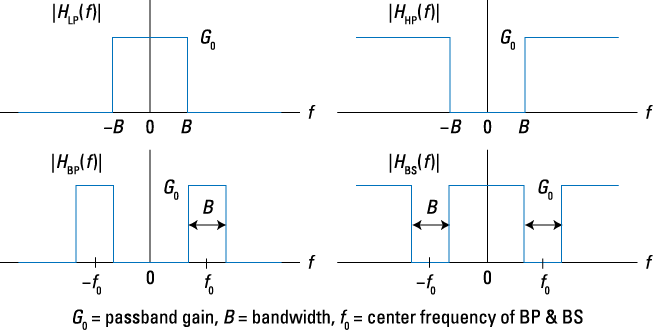
Figure 9-15: The frequency response of ideal filters: LP, HP, BP, and BS.
The passband corresponds to the band of frequencies passed by each of the filters. Ideal filters aren’t realizable, meaning you can’t actually build the filter; but they simplify calculations and give useful performance results during the initial phases of system design.
From the frequency response sketches of Figure 9-15, mathematical models for each filter type are possible. Consider this low-pass filter:
![]()
You can write the high-pass filter as 1 minus the low-pass filter, such as

Similar relationships exist for the band-pass and band-stop filters.
In all cases, the impulse response of an ideal filter is nonzero for t < 0, which, for an LTI system, means the filter is non-causal (see Chapter 5) — the filter output requires knowledge of future values of the input.
Realizable filters
You can approximate ideal filters with realizable filters, including the Butterworth, Chebyshev, and Bessel designs. At the heart of these three filter designs is a linear constant coefficient (LCC) differential equation having frequency response of the form
![]()
M and N are positive integers. The {ak} and {b} filter coefficients hold the keys to making the filter approximate one of the four ideal filter types. Figure 9-16 shows a third-order Chebyshev band-pass filter magnitude response.
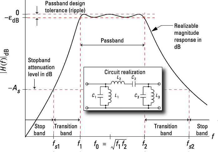
Figure 9-16: A third-order Chebyshev band-pass filter as an example of a realizable filter.
The bandwidth B in Figure 9-16 is ![]() , where f1 and f2 are the passband cutoff frequencies and fs1 and fs2 are the stopband cutoff frequencies. The filter stopband, where approximately no signals pass through the filter, is when
, where f1 and f2 are the passband cutoff frequencies and fs1 and fs2 are the stopband cutoff frequencies. The filter stopband, where approximately no signals pass through the filter, is when ![]() and
and ![]() . The center frequency is the geometric mean of the passband edges, or
. The center frequency is the geometric mean of the passband edges, or ![]() .
.