
Chapter 8
Line Spectra and Fourier Series of Periodic Continuous-Time Signals
In This Chapter
![]() Checking out the frequency domain of sinusoidal signals using line spectra
Checking out the frequency domain of sinusoidal signals using line spectra
![]() Navigating the Fourier series representation of periodic signals
Navigating the Fourier series representation of periodic signals
![]() Relating Fourier coefficients between waveform transformations
Relating Fourier coefficients between waveform transformations
Exploring the frequency distribution of a sinusoids-based signal is a first step into frequency domain analysis. I like to think of this topic in terms of music. If you play an instrument or even enjoy listening to music, you probably know that music is made up of sounds that occur at different frequencies. The rich harmony of multiple instruments playing together is full of different tones and frequencies. If you set out to electronically synthesize the sound produced by a particular instrument, knowing the frequency distribution for each playable note makes your task easier.
Line spectra and Fourier series function in a similar way to music; they team up to offer a spectral representation of a sinusoidal signal or a sum of many sinusoids. In other words, the amplitudes and frequencies of sinusoids produce the line spectra and are harmonically related.
All signals have a frequency distribution, or spectrum. But only some signals are periodic, meaning that they repeat with respect to time; the Fourier series applies only to periodic signals.
 You can thank Joseph Fourier, who lived from 1768 to 1830, for his pioneering work on periodic signals and the discovery of what’s known as Fourier series.
The Fourier series is a powerful mathematical tool, and it applies to multiple branches of engineering and mathematics. For electrical engineers, the Fourier series provides a way for you to represent any periodic signal as a sum of complex sinusoids via Euler’s formulas (see Chapter 2).
But the Fourier series isn’t a one-way street. After you analyze a periodic signal to get its Fourier coefficients, you can synthesize the signal by using the coefficients in a sum of complex sinusoids. The sinusoid frequencies are integer multiples (harmonics) of the fundamental frequency, which is the inverse of the waveform period.
 Getting lost in the mathematics and losing sight of the purpose of the Fourier series in signals and systems modeling is a common problem. I don’t want this to happen to you. I attempt to keep you focused on what the Fourier series provides, and I don’t dwell on tedious integrations to find the Fourier series coefficients. Computer tools can and do help you in this area.
In this chapter, I develop the Fourier series for common waveforms, including the square wave and pulse train. I also point out Fourier series properties you can use to find the Fourier coefficients of a new signal by just applying the corresponding coefficient transformation; no need to start from scratch. For an example of the Fourier series in action, check out the article on designing a frequency tripler at www.dummies.com/extras/signalsandsystems.
Sinusoids in the Frequency Domain
The signal ![]() is a function of time that has the parameters of amplitude, frequency, and phase. To view a sinusoid in the frequency domain means you consider the amplitude and the phase (such as complex number polar form) at the given frequency.
is a function of time that has the parameters of amplitude, frequency, and phase. To view a sinusoid in the frequency domain means you consider the amplitude and the phase (such as complex number polar form) at the given frequency.
For a single sinusoid, this may seem trivial; amplitude A at frequency f0 isn’t too exciting. But when you have multiple sinusoids and need to study the distribution or shape they form and find out how the distribution changes when the signal is passed through a system, things get more fun.
In this section, I point out how to construct the two-sided spectral representation of a signal that’s composed of multiple sinusoids. This is particularly useful when you first get started with spectral analysis because the two-sided spectra is closely related to the complex exponential Fourier series defined later in this chapter.
Initially, the two-sided spectra can be confusing because both positive and negative frequencies are represented; just keep in mind that a real cosine is characterized by a single nonnegative frequency.
I also cover one-sided spectra in this section, which displays only the nonnegative frequencies.
Viewing signals from the amplitude, phase, and frequency parameters
The three parameters of a sinusoid — amplitude, phase, and frequency — make up the three-legged stool of the frequency domain. To accommodate the two-sided spectra representation, I start with a complex sinusoid, because it’s more basic than the real sinusoid when viewed in terms of Euler’s formulas (covered in Chapter 2).
Consider this single complex sinusoid: ![]() .
.
To get a new view of this signal, construct a frequency-amplitude/phase pair to reveal that ![]() has spectral amplitude of A at
has spectral amplitude of A at ![]() and a spectral phase of
and a spectral phase of ![]() at
at ![]() .
.
 The spectral information is actually a complex number because it’s amplitude (magnitude) and phase in a polar representation. Catalog this information as a combined frequency-amplitude/phase pair with the notation
 ![]() . This is the humble beginning of frequency domain characterization.
. This is the humble beginning of frequency domain characterization.
For a more practical signal example, here’s the real sinusoid:
![]()
As a result of the Euler expansion of cosine, the frequency domain view of this ![]() is two frequency-amplitude/phase pairs:
is two frequency-amplitude/phase pairs: ![]() . The corresponding frequency-amplitude pairs are
. The corresponding frequency-amplitude pairs are ![]() , and the frequency-phase pairs are
, and the frequency-phase pairs are ![]() .
.
 A real sinusoid always has one positive frequency pair and one negative frequency pair. Don’t let that bother you. Negative frequencies are part of the mathematical baggage of signals and systems. Euler’s formula tells you that a real cosine or sine is composed of two complex exponentials; one has positive frequency and one has negative frequency. Real signals always have a symmetrical spectrum.
To generalize to multiple sinusoids, complex or real, take a look at this equation for K real sinusoids:
![]()
where ![]() for
for ![]() and
and ![]() for
for ![]() .
.
A further and significant observation regarding the ![]() notation is that
notation is that ![]() for real signals. To accommodate a possible waveform offset (level shift), just add the constant term
for real signals. To accommodate a possible waveform offset (level shift), just add the constant term ![]() , which is also known as the direct current (DC) term of the signal.
, which is also known as the direct current (DC) term of the signal.
A constant term also arises in the case of a zero frequency sinusoid. The spectral characterization of this signal consists of ![]() frequency-amplitude/phase pairs (the +1 is from the A0 term). If A0 < 0, you can write this in polar form as
frequency-amplitude/phase pairs (the +1 is from the A0 term). If A0 < 0, you can write this in polar form as ![]() (note
(note ![]() ).
).
Forming magnitude and phase line spectra plots
Frequency-amplitude pairs and frequency-phase pairs are graphically displayed as amplitude and phase line spectra plots, which you create by plotting vertical lines that start at 0 and end at the related amplitude or phase value; a horizontal offset represents the corresponding frequency.
Two-sided line spectra plots show both positive and negative frequencies. One-sided plots show only nonnegative frequencies. The amplitude values for the one-sided spectra are double those of the two-sided spectra for all but the DC term.
The one-sided plot applies only to real signals so instead of using Euler’s formula, you work directly with the real cosine ![]() , which has the one-sided frequency-amplitude/phase pair
, which has the one-sided frequency-amplitude/phase pair ![]() . The amplitude at f0 is A (not A/2) and the phase at f0 is
. The amplitude at f0 is A (not A/2) and the phase at f0 is ![]() .
.
The one-sided amplitude plot resembles the display produced by a spectrum analyzer (an instrument dedicated to displaying the one-sided amplitude spectrum of the input signal) or oscilloscope with spectrum display capabilities that you may find in a laboratory. An oscilloscope traditionally displays time-domain waveforms, but digital oscilloscopes can display the one-sided spectrum, using discrete-time signal processing techniques. A case study example in Chapter 16 explores discrete-time spectral analysis. These tools take you from math models to real measurements — great stuff.
 Example 8-1: Consider the real signal
 ![]()
![]() and plot the two-sided amplitude and phase line spectra by using the following three-step process:
and plot the two-sided amplitude and phase line spectra by using the following three-step process:
1. Expand ![]() into complex sinusoid pairs:
into complex sinusoid pairs:

2. Extract the five frequency-amplitude/phase pairs from the expansion of Step 1.
Five total pairs of the form ![]() exist:
exist:
![]()
3. Create plots.
A pencil-and-paper sketch gets the job done in this case. Figure 8-1 shows the double-sided amplitude and phase plots.
You can use Python to generate line spectra plots to check your work. I created the custom function line_spectra(fk,Xk,mode,sides=2) for this purpose. The ssd.py module contains the function, which you import at the IPython command prompt.
The function assumes the signal is real, so the inputs, which are of type ndarray, hold the nonnegative frequencies and complex amplitudes in fk and Xk, respectively. Setting sides=2 produces a two-sided plot and setting sides=1 produces a properly scaled one-sided plot.

Figure 8-1: Line spectra sketch amplitude (a) and phase (b) plots for a constant plus two real sinusoids signal.
Example 8-2: Suppose two idealized musical instruments play pure single-pitch tuning notes, each at a nominal frequency of 440 Hz (middle A in musical terms). Real instruments also produce overtones (harmonics) at integer multiples two and above of the fundamental pitch (frequency), but don’t worry about that for this example. If one instrument plays high (sharp) by 5 Hz and the other plays low (flat) by 5 Hz, you can model this scenario mathematically as a superposition of signals: ![]() .
.
The amplitude frequency pairs for this signal are ![]() .
.
You can plot both the waveform and the single-sided amplitude spectrum by using Python, as shown in Figure 8-2. Here, I chose to use a one-sided amplitude spectrum so you can see the difference in the amplitude scaling.
In [289]: t = arange(0,0.2,1/8000.)
In [290]: x = cos(2*pi*435*t)+cos(2*pi*445*t)
In [292]: plot(t,x)
In [297]: fk = array([435, 445])
In [298]: Xk = array([1/2., 1/2.])
In [299]: ssd.line_spectra(fk,Xk,'mag',sides=1)
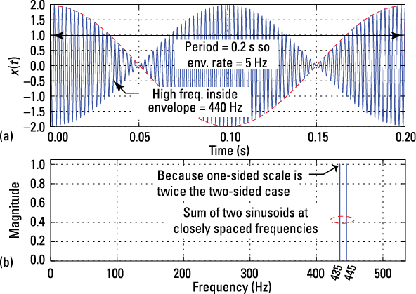
Figure 8-2: The waveform (a) and the single-sided line spectra (b) for a signal composed of 435- and 445-Hz sinusoids.
The waveform plot hints that the signal is made up of a high-frequency component and a low-frequency envelope oscillating at a 5-Hz rate. The line spectra plot makes it clear, however, that the signal is the sum of equal amplitude sinusoids that are closely spaced in frequency.
Another way of looking at ![]() is as a product of a 440-Hz sinusoid and a 5-Hz sinusoid. If you know the true mathematical form of
is as a product of a 440-Hz sinusoid and a 5-Hz sinusoid. If you know the true mathematical form of ![]() , you can approach the waveform plot with this trig identity (for more identities, see Chapter 2):
, you can approach the waveform plot with this trig identity (for more identities, see Chapter 2):
![]()
This identity works if you set ![]() and
and ![]() . Solving for u and v yields the following result:
. Solving for u and v yields the following result:

or
![]()
The average of the 435- and 445-Hz frequencies (or half the sum) is 440 Hz, and half the difference between 445- and 435-Hz frequencies is 5 Hz (the full difference is 10). Anyone listening to this music would hear a dominant sound (pitch) at 440 Hz and a beating sound (note) at 5 Hz. The two musicians could eliminate the beat note by tuning their instruments to each produce 440 Hz.
Working with symmetry properties for real signals
When ![]() is a real signal, the expansion into complex sinusoids always results in conjugate symmetry of the
is a real signal, the expansion into complex sinusoids always results in conjugate symmetry of the ![]() coefficients, meaning that if
coefficients, meaning that if ![]() ,
, ![]() , and
, and ![]() , then
, then ![]() .
.
![]() When looking at the double-sided amplitude spectrum, you see even symmetry because
When looking at the double-sided amplitude spectrum, you see even symmetry because ![]() .
.
![]() When looking at the double-sided phase spectrum, you see odd symmetry because
When looking at the double-sided phase spectrum, you see odd symmetry because ![]() .
.
Exploring spectral occupancy and shared resources
The frequency domain view brought by line spectra shows that signals occupy an interval of the frequency axis. The frequency interval is referred to as the signal bandwidth, in hertz. Each spectral line of a sinusoid has zero width, but the spectral line for information-bearing waveforms used in communications is replaced by a spectral shape, such as a rectangle, of width B Hz.
In communication systems, including radio, TV, wireless Internet, and cellular telephony, all signals occupy a band of frequencies centered on a carrier frequency, ![]() Hz. Even the sum of two equal amplitude sinusoids in Example 8-2 occupies a band of frequencies 10 Hz wide with
Hz. Even the sum of two equal amplitude sinusoids in Example 8-2 occupies a band of frequencies 10 Hz wide with ![]() Hz.
Hz.
Consider FM radio broadcasting, where stations are each assigned a carrier frequency from 87.5 to 108.0 MHz, spaced every 200 kHz. The spectral occupancy, or bandwidth, associated with an FM radio transmission is about ![]() kHz. In a given metro area or radio market, all 102 available channel frequencies aren’t assigned, but demand exists nationwide for more than 102 channels. Therefore, sharing of spectral bandwidth, a natural resource, is required; only a finite amount of usable bandwidth is available for today’s electronic technologies.
kHz. In a given metro area or radio market, all 102 available channel frequencies aren’t assigned, but demand exists nationwide for more than 102 channels. Therefore, sharing of spectral bandwidth, a natural resource, is required; only a finite amount of usable bandwidth is available for today’s electronic technologies.
Broadcast FM requires spectral sharing via frequency reuse. In terms of spectral occupancy, reuse means that two groups of users can both share the same spectrum as long as they’re spatially separated and they exercise power control. Power control means you transmit enough power to get the job done but with limits to allow sharing. Frequency reuse means that stations in Denver, Colorado, for example, use the same carrier frequency as stations in Colorado Springs, Colorado.
Denver and Colorado Springs are separated by about 80 miles; sharing via frequency reuse works because at carrier frequencies of around 100 MHz, the radio wave propagation is line of sight (LOS). LOS simply means the receiver needs to see the transmitter in a geometrical sense, because the radio waves don’t follow the curvature of the earth, nor do they bounce off the ionosphere. LOS isn’t sufficient for reception because the received signal power must overcome background noise.
Of the various classes of FM radio stations, the nominal coverage radius ranges from about 15 miles up to 50 miles. The 80 miles separating Colorado Springs and Denver is quite sufficient. Terrain is also a factor that can help.
Cellphones also employ frequency reuse. The cellular concept by its very name places users of a given locale into a cell. With a seven-cell reuse pattern, unique frequency bands are available for just seven cells. Not until you move three cells from your present location is the frequency band reused.
Personal music players with earbuds operate through a reuse scheme. Acoustical wave transmission of conversation and music uses the audio spectral bandwidth of 20 Hz to 20 kHz. The earbuds allow the acoustical propagation path to stay isolated for two side-by-side users, an example of audio spectrum sharing. In fact, earbuds themselves are transducers that convert electrical signals to acoustical sound pressure waves, much like the antenna hidden inside your cellphone sends and receives radio waves.
Establishing a sum of sinusoids: Periodic and aperiodic
A signal x(t) that’s modeled as a sum of sinusoids may be periodic or aperiodic. The line spectra exists in both cases, but the relationship between the individual sinusoid frequencies is tied to a common, or fundamental, frequency when x(t) is periodic. By fundamental frequency, I mean frequency f0 = 1/T0 exists, where T0 is the period of x(t). For x(t) periodic, you need the condition ![]() , where
, where ![]() , the period, is the smallest value, making the equality hold. If
, the period, is the smallest value, making the equality hold. If ![]() can’t be found, the signal is aperiodic. Flip to Chapter 3 for details on periodicity for continuous-time signals.
can’t be found, the signal is aperiodic. Flip to Chapter 3 for details on periodicity for continuous-time signals.
Take a look at this model:
![]()
With x(t) periodic, the frequencies ![]() are harmonically related to f0, which means that each fk is an integer multiple of f0. The harmonics have names. The first harmonic is the same as fundamental, f0. The second, third, and fourth harmonics are the frequencies 2f0, 3f0, and 4f0, respectively. The nth harmonic is nf0.
are harmonically related to f0, which means that each fk is an integer multiple of f0. The harmonics have names. The first harmonic is the same as fundamental, f0. The second, third, and fourth harmonics are the frequencies 2f0, 3f0, and 4f0, respectively. The nth harmonic is nf0.
If you have a sum of sinusoids signal, you can do the following:
1. Determine whether it’s periodic by seeing whether the greatest common divisor (GCD) of the frequencies exists.
If a zero frequency term is present, it isn’t part of this analysis. (Chapter 4 points out that the GCD is the fundamental frequency.) If the GCD of the signal frequencies doesn’t exist, then the signal is aperiodic.
2. After you have f0, find the harmonic number by dividing fk by f0.
Example 8-3: To verify periodicity, find the fundamental frequency. Also, find the harmonic numbers for the sinusoid frequencies of Examples 8-1 and 8-2. To get started, determine whether the signal is periodic and then find the harmonic number.
In Example 8-1, sinsuoids at 50 and 300 Hz are present. The fundamental frequency is GDC (50, 300) = 50 Hz. The harmonics present are 50/50 = 1 (also the fundamental) and 300/50 = 6 (the sixth).
In Example 8-2, sinusoids at 435 and 445 Hz are present. The fundamental frequency is GCD (435, 445) = 5 Hz. The harmonics present are 435/5 = 87 (the 87th) and 445/5 = 89 (the 89th).
Encountering lower-order harmonics is more common, but this isn’t always the case, as this example shows.
Example 8-4: Consider a square wave signal, which is a periodic signal that switches between ![]() every
every ![]() s (half period). Here’s a three-term sum of sinusoids approximation to a 100-Hz (
s (half period). Here’s a three-term sum of sinusoids approximation to a 100-Hz (![]() s) square wave with
s) square wave with ![]() :
:
![]()
The fundamental frequency is GCD (100, 300, 500) = ![]() Hz and
Hz and ![]() s. Because 100/100 = 1, 300/100 =3, and 500/100 = 5, this signal is composed of first, third, and fifth harmonic components.
s. Because 100/100 = 1, 300/100 =3, and 500/100 = 5, this signal is composed of first, third, and fifth harmonic components.
You may want to tweak the frequencies of the third and fifth harmonics to slightly modify the three-term approximation:

The ![]() doesn’t exist because irrational numbers are involved. The signal is now aperiodic. In decimal form, what was the third harmonic now resides at 299.998 Hz, and what was the fifth harmonic is now at 499.098 Hz. Figure 8-3 shows plots of the square wave (a), the three-term approximation (b), and the nearly periodic three-term approximation (c).
doesn’t exist because irrational numbers are involved. The signal is now aperiodic. In decimal form, what was the third harmonic now resides at 299.998 Hz, and what was the fifth harmonic is now at 499.098 Hz. Figure 8-3 shows plots of the square wave (a), the three-term approximation (b), and the nearly periodic three-term approximation (c).
The three-term square wave approximation is periodic, and this is visible in Figure 8-3b. By shifting the frequencies of the third and fifth harmonics ever so slightly, you can find the aperiodic character, but you need to look over a longer time span to see it. Figure 8-4 illustrates single-sided amplitude line spectra plots of the two three-term approximations.
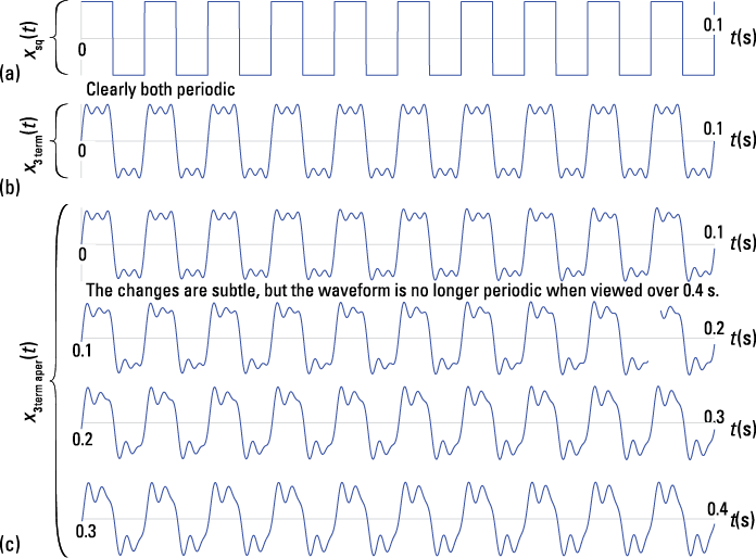
Figure 8-3: Plots of a 100-Hz square wave (a), a three-term sum of sinusoids approximation (b), and a three-term almost periodic (c).
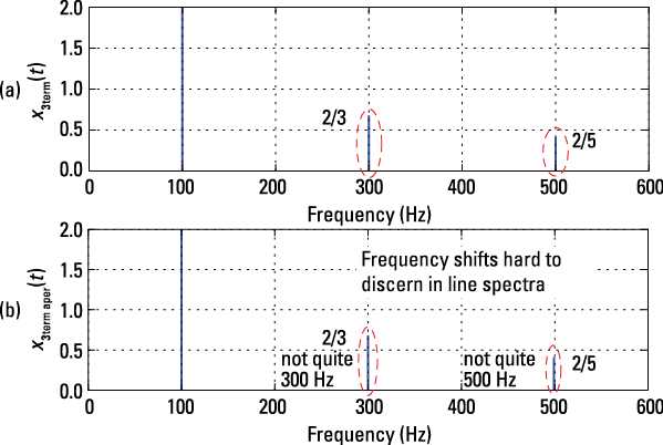
Figure 8-4: Single-sided line spectra amplitude plots of two three-term approximates: periodic (a) and aperiodic (b).
The take-away from this example is that a small deviation from periodicity can noticeably alter the time-domain waveform view, but it does little to the appearance of the corresponding line spectra. Figures 8-4a and 8-4b look virtually identical. Only by zooming in on the line spectrum near 300 Hz or 500 Hz in Figure 8-4b can you see the small frequency shift of the spectral lines that make the signal become aperiodic.
General Periodic Signals: The Fourier Series Representation
Periodic signals are a common occurrence in signals and systems but also in the broader sense of electronic devices. Timing and control signals are periodic as well as signals that act as carrier waves in wireless. Knowing the Fourier series representations broadens your understanding of how a signal interacts with other signals and systems. In this section, you work with the details of Fourier series analysis and synthesis for periodic signals. You analyze a periodic signal to find its Fourier coefficients, and later you synthesize the periodic signal by using the Fourier coefficient amplitude and phase values in a sum of complex sinusoids.
The sinusoid frequencies are harmonically related to the waveform fundamental frequency. When you bring together the harmonic frequencies and the Fourier coefficients found in the analysis phase, you have frequency-amplitude/phase pairs that you can use to construct the line spectra of this periodic waveform.
Finding the coefficients is the most tedious part of working with Fourier series. The tedium comes from integrations involving complex exponentials. In this section, I provide a series of examples, a table of coefficients for common waveforms, and also some useful Fourier coefficient properties.
Analysis: Finding the coefficients
To start, assume that the period of x(t) is T0 and the fundamental frequency is f0 = 1/T0. When using complex exponentials for the analysis, the synthesis formula takes this form:
![]()
where the Xn’s are the unknown Fourier coefficients you want to find and n is the harmonic number. Because I’m developing the complex exponential Fourier series, n takes on all integer values. The analysis formula that finds the ![]() ’s is
’s is
![]()
The T0 integration limit signifies that you can pick any ![]() second interval for
second interval for
the actual integration. Here, I assume you choose ![]() .
.
The ![]() coefficient, found when n = 0, is special because
coefficient, found when n = 0, is special because ![]()
![]() . The average value is also known as the DC value, which represents the constant offset value of the waveform. When a DC voltmeter is connected to this waveform, it displays X0.
. The average value is also known as the DC value, which represents the constant offset value of the waveform. When a DC voltmeter is connected to this waveform, it displays X0.
Developing the Fourier coefficient formula
Establishing the analysis formula requires some patience and a willingness to wade through integrations involving complex exponentials. Here are the five main steps to the proof:
1. Establish the orthogonality of the function ![]() when integrated over a
when integrated over a ![]() second interval.
second interval.
Function orthogonality means the dot (inner) product of two functions is 0. For vectors, the concept is more visual, because the vectors lie at right angles to one another and you can see the orthogonality.
The dot product for complex functions is defined as ![]() , where
, where ![]() denotes conjugation.
denotes conjugation.
2. Plug fn(t) and fm(t) into the integral:
![]()
For ![]() , the numerator is 0, making the integral 0. When
, the numerator is 0, making the integral 0. When ![]() , the integrand from the start is just 1 (find this in the beginning of the equation in Step 1), so the integral evaluates to
, the integrand from the start is just 1 (find this in the beginning of the equation in Step 1), so the integral evaluates to ![]() . The orthogonality condition that you just developed states the following:
. The orthogonality condition that you just developed states the following:
![]()
3. Use the orthogonality condition to set the stage for finding the coefficients. Write ![]() on the left and the synthesis formula on the right, and then multiply each side by
on the left and the synthesis formula on the right, and then multiply each side by ![]() and integrate over
and integrate over ![]() (lines 1 through 3 in the following equation):
(lines 1 through 3 in the following equation):

This simply represents Fourier’s Theorem, which states that x(t) can be represented as an infinite sum of sinusoids. Continue to work with the right side only in Step 4, ultimately solving for Xn.
4. Interchange the integral and the sum (I explain the consequences in the section “Synthesis: Returning to a general periodic signal, almost”).
Now, you reduce the integral on the inside by using the orthogonality property that you established in Step 2. Only the ![]() term survives:
term survives:

5. Rearrange a bit by dividing both sides by ![]() and changing m to n everywhere:
and changing m to n everywhere:
![]()
Voilà! Now you have the formula.
Fourier series coefficients are unique! If you can find the coefficients by looking at the math form of the waveform and knowing how the Fourier series itself is assembled, then you’re done — no integration required. So if the given x(t) is composed of sine and cosine terms, you can find the Xn coefficients by setting x(t) equal to the general Fourier series expansion and then matching up terms. Here are the steps for this process:
1. Find the fundamental frequency of the cosine terms that make up x(t).
2. Identify the harmonic numbers of the terms.
If n = 0 is present, then you identified the X0 coefficient.
3. Convert all terms to cosine form by using trig identities of Euler’s formulas.
4. Expand each cosine into complex exponentials by using Euler’s formula for cosine.
5. Equate the magnitude and phase values of the factors from the complex exponential and equate them to the corresponding Xn values at the given harmonic number n.
Example 8-5: Consider the equation ![]()
![]() .
.
To find the Fourier series expansion by inspection, work through the five steps to find the Xn coefficients. In Step 1, GCD(20, 30) = 10, so f0 = 10 Hz. In Step 2, the harmonic numbers are 20/10 = 2 and 30/10 = 3. There’s no n = 0 term. Step 3 isn’t needed here, because the terms are already in cosine form. In Step 4, you expand the cosine terms by using Euler’s formula for cosine.
![]()
Finally, in Step 5, you match the magnitude and phase values identified in Step 4 with the Xn values for ![]() and
and ![]() . All other Xn terms are zero.
. All other Xn terms are zero.
![]()
As promised, the Fourier coefficients — all four of them — pop out without using any integration.
Synthesis: Returning to a general periodic signal, almost
After synthesizing for ![]() from the
from the ![]() coefficients, the N term synthesis approximation is
coefficients, the N term synthesis approximation is ![]() .
.
As ![]() , you may expect the sum to approach
, you may expect the sum to approach ![]() , but I have some sad news: For some signals, the synthesis doesn’t return the original signal — not in a point-by-point convergence sense. If
, but I have some sad news: For some signals, the synthesis doesn’t return the original signal — not in a point-by-point convergence sense. If ![]() contains jumps, as in the square wave defined in Example 8-3, the synthesis formula converges to the average of the left- and right-hand limits. For the square wave that jumps from –A to A or A to –A, the average is 0.
contains jumps, as in the square wave defined in Example 8-3, the synthesis formula converges to the average of the left- and right-hand limits. For the square wave that jumps from –A to A or A to –A, the average is 0.
The good news is that, with the exception of ideal mathematical modeling, a physical square wave doesn’t actually contain a jump, so the lack of pointwise convergence isn’t an issue in the real world.
A second convergence issue, again exemplified by the square wave, is that the N term sum oscillates around the true waveform value (![]() ) either side of the jump. The maximum overshoot value is about 9 percent, and it decays as you get farther away from the jump. Increasing N doesn’t eliminate the 9 percent peak overshoot; it simply increases the oscillation rate. See Figure 8-5 for examples of the square wave as N steps through values of 3, 9, 31, and 101. For the case of
) either side of the jump. The maximum overshoot value is about 9 percent, and it decays as you get farther away from the jump. Increasing N doesn’t eliminate the 9 percent peak overshoot; it simply increases the oscillation rate. See Figure 8-5 for examples of the square wave as N steps through values of 3, 9, 31, and 101. For the case of ![]() , just the jump interval
, just the jump interval ![]() is shown.
is shown.
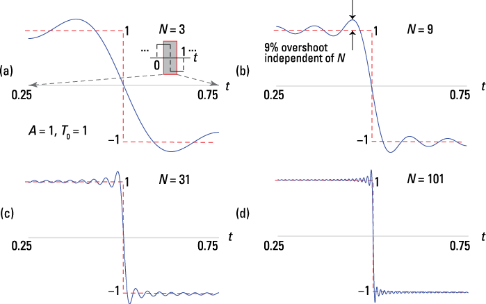
Figure 8-5: Square wave convergence ringing as N is increased from 3 (a), 9 (b), 31 (c), and 101 (d) in the synthesis approximation.
Checking out waveform examples
In this section, I point out how to derive Fourier series coefficients for common periodic waveforms, and I develop numerical calculations of the coefficients. Pay particular attention to the details of how to simplify the integration results into a compact coefficient formula as a function of harmonic number n.
Square wave and pulse train
Over one T0 period, the periodic pulse train is mathematically described by this equation:
![]()
where ![]() controls the pulse width. A sketch of the signal is shown in Figure 8-6.
controls the pulse width. A sketch of the signal is shown in Figure 8-6.
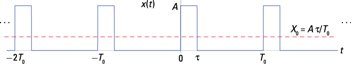
Figure 8-6: A periodic pulse train that specializes to a square wave when ![]() .
.
By setting ![]() , you get the square wave that was defined in Example 8-3. To find a formula for the
, you get the square wave that was defined in Example 8-3. To find a formula for the ![]() coefficients, use this equation:
coefficients, use this equation:
![]()
You can stop here, but it’s really worth the extra effort to reduce the formula to a more compact form. So I suggest forming a sine from the numerator by
factoring ![]() outside both terms:
outside both terms:

In the last line, I introduce a handy function:
![]()
Most scientific computing environments, including PyLab, define the sinc( ) function. You can find sinc(0) by using L’Hôspital’s rule, which gives you a means to evaluate the limit of 0/0 by taking derivatives of the numerator and denominator before taking the limit:
![]()
In [518]: sinc(0)
Out[518]: 1.0
In [519]: sinc(0.5)
Out[519]: 0.6366
By setting ![]() , you can get the special case of the square wave. Although not immediately obvious, you can show that
, you can get the special case of the square wave. Although not immediately obvious, you can show that

When taken together, ![]() for n odd and 0 for n even but not equal to 0. Especially note the even harmonics are 0 for the square wave.
for n odd and 0 for n even but not equal to 0. Especially note the even harmonics are 0 for the square wave.
Example 8-6: Plot the amplitude and phase line spectra for a pulse train having ![]() . You can use the Python function
. You can use the Python function line_spec() to create the plots and the IPython-created function pt_Xn() to generate the coefficients, as the following code and Figure 8-7 show.
In [520]: def sq_Xn(N,f0tau): # custom function for
...: Xk = zeros(N+1)+0j # pulse train Xn
...: fk = arange(0,N+1) # coefficient generation
...: for k in range(N+1):
...: Xk[k] = f0tau*sinc(k*f0tau)*exp(-1j*pi*k*f0tau)
...: return Xk, fk
In [521]: Xn, fn = sq_Xn(25, 0.125) Sq-wv Xn's and fn's
In [522]: ssd.line_spectra(fn,Xn,'mag')#two-sided plots
In [523]: ssd.line_spectra(fn,Xn,'phase') # mag & phase
The magnitude of the coefficients is proportional to ![]() , so the shaping of the amplitude lines consists of a main lobe between
, so the shaping of the amplitude lines consists of a main lobe between ![]() and side lobes spaced at multiples of
and side lobes spaced at multiples of ![]() . Spectral nulls always occur at integer multiples of
. Spectral nulls always occur at integer multiples of ![]() Hz; in this case, 8, 16, and 24 are shown.
Hz; in this case, 8, 16, and 24 are shown.
For the square wave, ![]() , so the nulls occur at 2, 4, 6, . . . Hz, the even harmonics.
, so the nulls occur at 2, 4, 6, . . . Hz, the even harmonics.
The minimum line spacing is controlled by ![]() ; here, it’s 1 Hz. The
; here, it’s 1 Hz. The ![]() in the coefficients formula creates a negative slope of
in the coefficients formula creates a negative slope of ![]() with respect to the line frequency
with respect to the line frequency ![]() in the phase spectral lines. Both plots continue beyond
in the phase spectral lines. Both plots continue beyond ![]() Hz.
Hz.
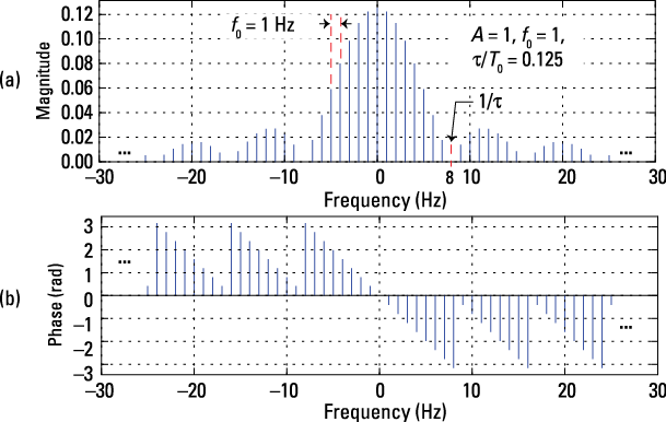
Figure 8-7: The amplitude (a) and phase line spectra (b) for a pulse train with ![]()
![]()
![]() .
.
Triangular wave
Another fundamental periodic waveform is the triangular wave. Over one period, the mathematical form is given by this equation:
![]()
Figure 8-8 shows a sketch of the signal.
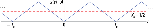
Figure 8-8: A triangular wave with period ![]() .
.
Start by finding the ![]() coefficient, and keep in mind that for n = 0, you just need to find the area of x(t) over a period times 1/T0:
coefficient, and keep in mind that for n = 0, you just need to find the area of x(t) over a period times 1/T0:
![]()
The dashed line in Figure 8-8 is located at A/2, which represents the average value.
Next, find the general integral for the ![]() coefficients by breaking the integral into two parts:
coefficients by breaking the integral into two parts:
![]()
To evaluate this integral, you must use integration by parts or use the integral table in Chapter 2. Specifically,
![]()
A third option is to use a computer algebra system (CAS), such as the open source CAS Maxima or the CAS capabilities Python via symPy. Using wxMaxima, which is the GUI version of Maxima, you come up with the following:
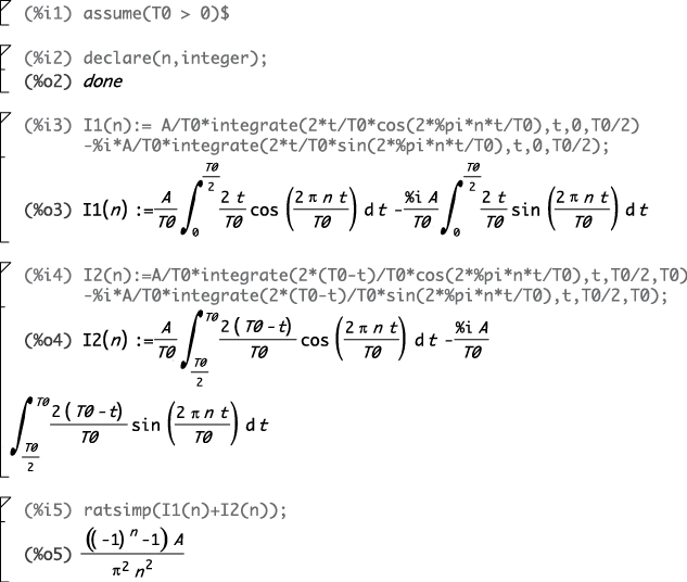
When using Maxima, I found it helpful to first use Euler’s formula to break the complex exponential into cosine and sine terms. Doing so helps Maxima simplify the result. The ![]() term reduced is 0 for n even (except 0) and –2 for n odd. Finally, you get this solution:
term reduced is 0 for n even (except 0) and –2 for n odd. Finally, you get this solution:

As with the square wave, the even harmonic terms are 0. For integration manipulation practice, I recommend that you verify these Xn values by using the integration table formula.
Example 8-7: The spectral line distribution is, in general, different for each waveform, even when both waveforms have the same fundamental frequency. In this example, I want you to see the differences between the square wave and the triangle wave when ![]() Hz in both waveforms. Compare the amplitude line spectra in dB, relative to the strength of the fundamental component, out to the 15th harmonic. Use a single-sided display format. Also compare the synthesis of the triangle wave, using up to the 3rd and 15th harmonics.
Hz in both waveforms. Compare the amplitude line spectra in dB, relative to the strength of the fundamental component, out to the 15th harmonic. Use a single-sided display format. Also compare the synthesis of the triangle wave, using up to the 3rd and 15th harmonics.
The functions tri_Xn(N) and sq_Xn(N) are defined in IPython (see Example 8-6) to generate Xn and fn arrays for plotting by using line_spec(). You get a normalized dB scale for the y-axis of the line spectra amplitude by taking ![]() for the double-sided display (
for the double-sided display (sides=2) and adding an additional 6.02 dB for the single-sided display (sides=1), because scaling by two in dB is the same as adding ![]() . By setting
. By setting mode='magdBn' in line_spec(), you can get the normalized dB displays of Figure 8-9.
Here are the IPython abbreviated commands:
In [532]: Xn_sq, fn = sq_Xn(15) # Sq-wv Xn's and fn's
In [533]: Xn_tri, fn = tri_Xn(15) # Tri Xn's and fn's
In [534]: ssd.line_spectra(10*fn,Xn_sq,'magdBn',sides=1)
In [535]: ssd.line_spectra(10*fn,Xn_tri,'magdBn',sides=1)
For both waveforms, only the odd harmonics are present (except for DC, the ![]() line). The added smoothness of the triangle wave (which is actually the integral of the square wave) makes the spectral lines roll off as
line). The added smoothness of the triangle wave (which is actually the integral of the square wave) makes the spectral lines roll off as ![]() versus just
versus just ![]() for the square wave.
for the square wave.
Both signals have just the odd harmonics present. From an interference standpoint, the square wave harmonics can be a problem. For instance, consider a PC with a clock frequency of 2 GHz. A clock signal in digital logic is like a square wave. The third and fifth harmonics drop less than 15 dB from the fundamental level and are at frequencies of ![]() and
and ![]() GHz, respectively. You need to make sure these high frequencies and the baseline frequency don’t radiate outside the computer and interfere with other electronic devices.
GHz, respectively. You need to make sure these high frequencies and the baseline frequency don’t radiate outside the computer and interfere with other electronic devices.

Figure 8-9: Line spectra in normalized dB for a triangle wave (a) and a square wave (b).
The square wave doesn't converge well at the jump points (check out a visual in Figure 8-5). The triangle wave doesn't contain jumps so you may expect better convergence when using the N-term Fourier synthesis formula. Find out whether that's what you really get by using the Python function fs_approx() (in the code module ssd.py) to plot the Fourier series synthesis approximation, using ![]() . This function implements the synthesis formula provided at the beginning of the section "Analysis: Finding the coefficients," earlier in this chapter. The results are available in Figure 8-10.
. This function implements the synthesis formula provided at the beginning of the section "Analysis: Finding the coefficients," earlier in this chapter. The results are available in Figure 8-10.
In [583]: t = arange(0,.2,.001) # time axis for plot
In [584]: Xn_tri3, fn = tri_Xn(3) # tri coeff. N=3
In [585]: Xn_tri15, fn = tri_Xn(15) # tri coeff. N=15
In [593]: x_app3 = ssd.fs_approx(Xn_tri3,10*fn,t)
In [594]: plot(t,x_app3) # plot x(t) for N = 3
In [600]: x_app15 = ssd.fs_approx(Xn_tri15,10*fn,t)
In [601]: plot(t,x_app15) # plot x(t) for N = 15
Yes, your expectations about the convergence panned out. The Fourier series does a good job of approximating the true triangle signal by using just a few terms. This is consistent with the rapid roll-off rate of the amplitude spectra and lack of jumps. It’s nice when things work out well after a long day of work.
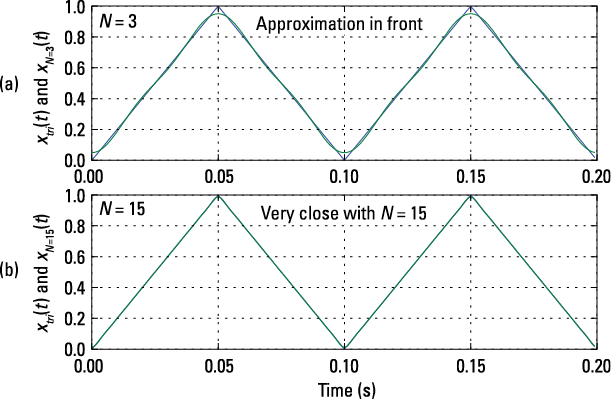
Figure 8-10: Fourier series approximation to a triangle wave, using up to the 3rd harmonic (a) and up to the 15th harmonic (b).
Working problems with coefficient formulas and properties
When solving problems with Fourier series analysis, a table of Xn values for popular waveforms can be quite helpful. The information in this section can help you make quick work of problems. Figure 8-11 shows you the complex exponential Fourier series coefficients for five periodic waveforms.
Before you begin working a problem, I suggest that you get familiar with some of the most significant Fourier series coefficient properties. I describe a few in this section. Time and level shifting properties, for example, may allow you to easily find the Fourier coefficients of your signal if it’s related to a signal previously analyzed. Figure 8-11 is also useful in this case. A set of symmetry properties explain the character of the Fourier coefficients; that’s why they’re purely real or imaginary or why the even index coefficients are zero. If your signal has one of these symmetries, you can use these properties to, in part, validate your solution.
![]() DC level shifting and gain scaling: Assuming that
DC level shifting and gain scaling: Assuming that ![]() has Fourier series coefficients
has Fourier series coefficients ![]() , consider the signal
, consider the signal ![]() .
.
You can show that these are the Fourier series coefficients of ![]() :
:
![]()
![]() Time shifting: Assuming that
Time shifting: Assuming that ![]() has Fourier series coefficients
has Fourier series coefficients ![]() , consider the time-shifted signal
, consider the time-shifted signal ![]() .
.
You can show that the Fourier series coefficients of ![]() are
are ![]() .
.
With the time shifting and level sifting/gain scaling properties, you can do almost anything! These properties are all about helping you avoid the tedious and error prone nature of the Fourier series coefficients integral (covered earlier in the section “Analysis: Finding the coefficients”). At the very least, these properties can help you check your work.
If the waveform of interest looks like something you’ve seen before, perhaps in Figure 8-11 or an example problem from another source, chances are good that the combination of these two properties will allow you to reuse the known coefficient formulas.
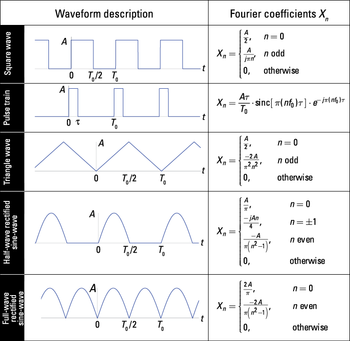
Figure 8-11: A table of common Fourier series coefficient formulas.
Example 8-8: Consider a triangular wave that’s symmetrical about ![]() and has symmetrical amplitude swings of
and has symmetrical amplitude swings of ![]() . Mathematically, the triangular wave has this form:
. Mathematically, the triangular wave has this form:

If you compare this description with the triangular wave of the table in Figure 8-11, it appears that ![]() .
.
To be sure, draw a sketch like the one shown in Figure 8-12.
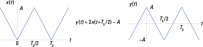
Figure 8-12: Transforming the triangular wave of the table in Figure 8-11 into the form of y(t).
The time shift is ![]() so
so ![]() .
.
Now, find the corresponding coefficients under the transformation, ![]() :
:
![]()
Plug in the specific coefficients from the table in Figure 8-11 for ![]() result in
result in ![]() and for n odd:
and for n odd:
![]()
This reveals your solution in a far easier process than working with the integration formula for ![]() :
:

Waveform symmetry
In the section “Working with symmetry properties for real signals,” I cover the symmetry of coefficients when ![]() is real. Now I describe the impact of waveform symmetry on the coefficients. Here are three properties to consider:
is real. Now I describe the impact of waveform symmetry on the coefficients. Here are three properties to consider:
![]() Even function of time: If
Even function of time: If ![]() , then
, then ![]() . That is,
. That is, ![]() .
.
![]() Odd function of time: If
Odd function of time: If ![]() , then
, then ![]() , or
, or ![]() .
.
![]() Odd half-wave symmetry: If
Odd half-wave symmetry: If ![]() , then
, then ![]() .
.
Odd half-wave symmetry stands far above being even and odd functions of time in significance and usefulness because it’s a big deal when a signal spectrum contains only odd harmonics. When both the square wave and triangle wave exhibit odd half-wave symmetry, the even harmonics are zero (a situation that exists in the analysis of the section “Checking out waveform examples”). Switching signals in electronics, particularly clock waveforms used in digital computers, exhibit this property. This property is also taken advantage of in the waveform generation system described later in the section “Application Example: Frequency Tripler.”
Parseval’s theorem
Parseval’s theorem relates the power in the periodic signal ![]() to the Fourier series coefficients:
to the Fourier series coefficients:
![]()
Consistent with the power calculations that I develop in Chapter 3, I assume a 1-ohm system in this case. This means x(t) appears across a 1-ohm resistor, so P has units of watts. From the sum terms in the power expression, the power in each complex sinusoid term is ![]() . As a result of the coefficient symmetry for real signals, or
. As a result of the coefficient symmetry for real signals, or ![]() , it follows that the power in each real cosine is
, it follows that the power in each real cosine is ![]() for n > 0. The n = 0 term has power
for n > 0. The n = 0 term has power ![]() .
.
Example 8-9: Consider a square wave of the form shown in the first row of Figure 8-11. What fraction of the total signal power resides in the fundamental frequency? Note that the amplitude A and period T0 doesn’t need to be defined because you’re finding the fraction of total power, meaning the quantity of interest is dimensionless.
The most effective way to work this problem is to make use of Parseval’s theorem. Complete the solution in three steps:
1. Find the total signal power, P, using the time-domain formula.
Integrate over one period, as the formula states,
![]()
2. Determine the power in the fundamental frequency by finding the power in the n = 1 and n = –1 complex sinusoids or simply ![]() .
.
From the square wave coefficients entry of Figure 8-11, you can write
![]()
3. Form the ratio Pfundamental/P:
![]()
Find an example of Fourier series in action at www.dummies.com/extras/signalsandsystems.