
Chapter 6
Advanced Fault Analysis with Techniques from Cryptanalysis
As introduced in Chapter 5, fault analysis causes a faulty computation during the encryption process. The basic differential fault analysis (DFA) exploits the difference of the correct computation and the faulty computation and recovers the key using the principle of differential cryptanalysis. Once the desired fault is injected to the middle of the computation, the remaining analysis is basically the same as the theoretical cryptanalysis. In fact, many of the techniques developed for the theoretical cryptanalysis can also be used in fault analysis.
On the contrary, fault analysis requires to deal with several problems that do not appear in the theoretical cryptanalysis. For example, in the theoretical differential cryptanalysis, the value of input difference can be chosen by the attacker because the input difference is the one between two plaintexts that are chosen by the attacker in the chosen plaintext attack model. On the other hand, in the DFA, the value of input difference cannot be chosen by the attacker because the fault injection cannot be controlled by the attacker in the random fault model.
The purpose of this chapter is applying the techniques for the theoretical cryptanalysis to fault analysis in order to optimize the attack. There are two approaches of optimizing fault analysis.
- Relaxing the fault model: This is very important for fault analysis. To recover the key in practice, the fault model must match the effect that can actually be caused by physical fault injections. In general, the more expensive devices are used, the more accurate and complicated faults can be injected. Relaxing the fault model is meaningful in the sense that fault analysis becomes more feasible.
- Reducing the cost to recover the key: Different from theoretical cryptanalysis, the goal of the fault analysis is recovering the key in practice, rather than finding a shortcut attack, which is infeasible but theoretically faster than the brute force attack. For example, for AES with a 128-bit key, the attack with a computational cost of
 AES operations is regarded as a vulnerability of the AES algorithm in the sense of theoretical cryptanalysis, whereas operating
  AES encryptions are computationally infeasible withthe current computation resources, and thus is not important in the sense of fault analysis. There seems to exist a consensus in the current cryptographic community that performing
  operations is hard or at least too expensive for fault analysis. In another aspect, a small number of fault injections is very important for fault analysis. This is because fault analysis is an active attack, that is, it actually gives unusual physical impact to the device. The device can be broken by such a physical impact, and then the attacker faces two problems:
- 1. The attacker cannot continue the key recovery procedure.
- 2. The attacker may be detected by the owner of the device that the device is being attacked.
6.1 Optimized Differential Fault Analysis
The basic DFA in Chapter 5 only introduced the basic concept, but did not explain the full description of the attack or advanced techniques for optimization. This section aims to optimize DFA.
6.1.1 Relaxing Fault Model
Recall Figure 5.75 in Chapter 5, which is a differential propagation in basic DFA. The assumed fault model in this attack is as follows:
1 byte of fault is injected at the beginning of the 8th round of AES-128. The faulty byte position is known to attackers, while the faulty value is not known to attackers.
As mentioned before, relaxing the fault model is important for fault analysis, hence optimized DFA relaxes it as follows:
1 byte of fault is injected at the beginning of the 8th round of AES-128. The faulty byte position is unknown to attackers. The faulty value, either.
The assumption is relaxed in optimized DFA, that is, the faulty byte position becomes unknown to the attackers. This is very meaningful for applications in practice. The attacker indeed cannot detect the faulty byte position after some physical impact is added to the device. Several experimental reports also indicate that causing the fault on a fixed target byte position with probability 1 is infeasible. Hence, DFA that can deal with unknown faulty byte position is practically meaningful.
6.1.1.1 Obtaining 
The generation of correct and faulty ciphertexts is basically the same as basic DFA. The attacker assumes that a plaintext P is encrypted twice. For the first time, the attacker observes the corresponding ciphertext C without injecting fault, and achieves a pair of ![]() . For the second time, the attacker injects a 1-byte fault at the beginning of round 8, and obtains the corresponding faulty ciphertext
. For the second time, the attacker injects a 1-byte fault at the beginning of round 8, and obtains the corresponding faulty ciphertext ![]() . Note that the timing of the fault injection (the beginning of round 8) should be measured before the analysis. It is widely known that the timing can be measured quite accurately. In summary, the attacker obtains a pair of
. Note that the timing of the fault injection (the beginning of round 8) should be measured before the analysis. It is widely known that the timing can be measured quite accurately. In summary, the attacker obtains a pair of ![]() and the faulty ciphertexts
and the faulty ciphertexts ![]() generated by the fault satisfying the fault model.
generated by the fault satisfying the fault model.
6.1.2 Four Classes of Faulty Byte Positions
On the basis of this fault model, the differential propagation in Figure 5.75 is reviewed. The new differential propagation is depicted in Figure 6.1. From the new fault model, the 1-byte fault is injected at state ![]() but its position is unknown. The straightforward method for the attacker is guessing the faulty byte position exhaustively, and performing the basic DFA for all the guesses. Because the state consists of 16 bytes, the number of guesses is at most 16, which roughly concludes that DFA with the new fault model can finish with 16 times as much cost as basic DFA.
but its position is unknown. The straightforward method for the attacker is guessing the faulty byte position exhaustively, and performing the basic DFA for all the guesses. Because the state consists of 16 bytes, the number of guesses is at most 16, which roughly concludes that DFA with the new fault model can finish with 16 times as much cost as basic DFA.
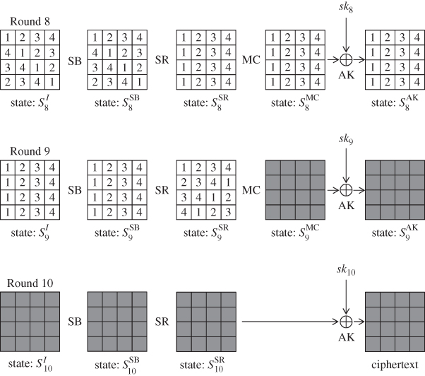
Figure 6.1 Differential propagation for four classes of faulty byte position at 
The attack cost can be improved more. The 16 candidates of the faulty byte position are divided into the following four classes:
- Class 1: byte positions 0, 5, 10, and 15.
- Class 2: byte positions 3, 4, 9, and 14.
- Class 3: byte positions 2, 7, 8, and 13.
- Class 4: byte positions 1, 6, 11, and 12.
The numbers in each state in Figure 6.1 show the differential propagation for each class.
Four positions in each class can be analyzed with exactly the same procedure. Therefore, the attack cost can be at most four times as much as basic DFA. Suppose that the fault is injected to any 1 byte of ![]() . The corresponding active byte position after the
. The corresponding active byte position after the ![]() operation is 1 byte of
operation is 1 byte of ![]() , and the corresponding active byte position after the
, and the corresponding active byte position after the ![]() operation is 1 byte of
operation is 1 byte of ![]() . The important fact is that in any of the four cases, the input state to the
. The important fact is that in any of the four cases, the input state to the ![]() operation,
operation, ![]() , contains 1 active byte in the left most column. The MDS property of the
, contains 1 active byte in the left most column. The MDS property of the ![]() operation guarantees that the number of active bytes in the input and the output columns is greater than or equal to 5. Therefore, in any of the four cases, all the 4 bytes in the left most column (labeled as “1”) of
operation guarantees that the number of active bytes in the input and the output columns is greater than or equal to 5. Therefore, in any of the four cases, all the 4 bytes in the left most column (labeled as “1”) of ![]() are active. In the remaining part of the attack, only the information of 4 active byte positions in
are active. In the remaining part of the attack, only the information of 4 active byte positions in ![]() is used. Thus, 4 faulty byte positions in class 1 are equivalent for the analysis. Similarly, 4 faulty byte positions in each of the other classes can be shown to be equivalent for the analysis. Classes 2, 3, and 4 contain 4 active bytes labeled as “2,” “3,” and “4” at
is used. Thus, 4 faulty byte positions in class 1 are equivalent for the analysis. Similarly, 4 faulty byte positions in each of the other classes can be shown to be equivalent for the analysis. Classes 2, 3, and 4 contain 4 active bytes labeled as “2,” “3,” and “4” at ![]() , respectively.
, respectively.
6.1.3 Recovering Subkey Candidates of 
The key recovery procedure is iterated four times by exhaustively guessing the class of the faulty byte position. In the following, the analysis for class 1 is explained.
DFA first aims to recover the last subkey ![]() . The overall picture for this process is shown in Figure 6.2.
. The overall picture for this process is shown in Figure 6.2.

Figure 6.2 Recovery of 4 bytes of  for class 1
The attacker analyzes the difference of two encryption processes, one is for computing C and the other is for computing ![]() . When the faulty byte position at
. When the faulty byte position at ![]() belongs to class 1, 4 bytes of
belongs to class 1, 4 bytes of ![]() have nonzero difference. From the MDS property of the
have nonzero difference. From the MDS property of the ![]() operation, all bytes of
operation, all bytes of ![]() have nonzero difference. The number of possible differences for each input column is
have nonzero difference. The number of possible differences for each input column is ![]() , thus the number of possible differences for each output column is also
, thus the number of possible differences for each output column is also ![]() . Because the
. Because the ![]() operation does not affect the difference, the same difference is preserved until
operation does not affect the difference, the same difference is preserved until ![]() , which is equivalent to
, which is equivalent to ![]() . From the analysis so far, the input difference to the S-box in round 10,
. From the analysis so far, the input difference to the S-box in round 10, ![]() , is determined uniquely for each possibility of
, is determined uniquely for each possibility of ![]() .
.
The output difference from the S-box in round 10, ![]() , can be computed from the ciphertext pair
, can be computed from the ciphertext pair ![]() . C and
. C and ![]() are known values to the attacker, thus its difference
are known values to the attacker, thus its difference ![]() can be computed. During the backward computation, the values are soon hidden by the last subkey XOR with
can be computed. During the backward computation, the values are soon hidden by the last subkey XOR with ![]() , however, the difference can still be traced. In fact
, however, the difference can still be traced. In fact ![]() can be computed by
can be computed by ![]() .
.
As explained in differential cryptanalysis in Section 4.2, for a pair of input and output differences for S-box, the paired values can be obtained using the differential distribution table (DDT) of the AES S-box. The idea was introduced in Figure 4.22 as a technique for driving key suggestions without guess. For DFA, subkey candidates for ![]() are derived with this technique, and the analysis is processed column by column. The analysis for the left most column is stressed by bold line in Figure 6.2.
are derived with this technique, and the analysis is processed column by column. The analysis for the left most column is stressed by bold line in Figure 6.2.
How to derive the paired values of the left most column of ![]() is explained below. The 4-byte output difference is uniquely fixed by
is explained below. The 4-byte output difference is uniquely fixed by ![]() , and there are about
, and there are about ![]() choices for the 4-byte input difference of
choices for the 4-byte input difference of ![]() . According to the DDT of the AES S-box, a pair of randomly determined input and output differences of the S-box has
. According to the DDT of the AES S-box, a pair of randomly determined input and output differences of the S-box has
- two solutions with probability 126/256,
- four solutions with probability 1/256, and
- no solution with probability 129/256.
For the sake of simplicity, the above can be roughly approximated such that a pair of randomly determined input and output differences of the S-box has two solutions with probability 1/2, otherwise, the pair does not have a solution. A pair of input and output differences is called “matched” when they have solutions to satisfy its propagation. For each of the ![]() choices of
choices of ![]() , the existence of the solution to achieve
, the existence of the solution to achieve ![]() is checked with DDT. Because the matchis examined for 4 bytes, the probability that there exist solutions for all bytes is
is checked with DDT. Because the matchis examined for 4 bytes, the probability that there exist solutions for all bytes is ![]() . Once the match is verified for 4 bytes, 4 byte values can be fixed to any of the solutions. The number of solution for each byte is 2, and any combination of the solutions of 4 bytes can make a valid value of
. Once the match is verified for 4 bytes, 4 byte values can be fixed to any of the solutions. The number of solution for each byte is 2, and any combination of the solutions of 4 bytes can make a valid value of ![]() . Thus,
. Thus, ![]() solutions of
solutions of ![]() are obtained from each match. In total,
are obtained from each match. In total, ![]() choices of the input difference can match in all of the 4 bytes, and
choices of the input difference can match in all of the 4 bytes, and ![]() solutions are obtained, which yields
solutions are obtained, which yields ![]() values of the left most column of
values of the left most column of ![]() .
.
![]() values
values ![]() will move to
will move to ![]() by the subsequent
by the subsequent ![]() operation. Finally,
operation. Finally, ![]() candidates of
candidates of ![]() can be computed as
can be computed as
6.1.3.1 Obtaining Subkey Candidates for Entire 
After obtaining ![]() candidates of
candidates of ![]() , the analysis is performed for the other columns independently. The analysis is almost the same. The only difference is that the input difference comes from a different byte position of
, the analysis is performed for the other columns independently. The analysis is almost the same. The only difference is that the input difference comes from a different byte position of ![]() , which does not give significant impact to the attack procedure. Thus,
, which does not give significant impact to the attack procedure. Thus, ![]() candidates of
candidates of ![]() ,
, ![]() candidates of
candidates of ![]() , and
, and ![]() candidates of
candidates of ![]() are obtained by iterating the same procedure for the second, third, and the fourth column of the
are obtained by iterating the same procedure for the second, third, and the fourth column of the ![]() operation in the last round.
operation in the last round.
6.1.3.2 Recovery of the Original Key 
The correct value of ![]() is now limited to
is now limited to ![]() candidates per diagonal, which makes
candidates per diagonal, which makes ![]() candidates of the entire
candidates of the entire ![]() . The correctness of those
. The correctness of those ![]() candidates can be verified by the exhaustive search. The attacker uses the pair of
candidates can be verified by the exhaustive search. The attacker uses the pair of ![]() . For each of the
. For each of the ![]() candidates of
candidates of ![]() , the attacker computes the corresponding
, the attacker computes the corresponding ![]() by inverting the key schedule function. The correctness of the candidate can be checked by matching
by inverting the key schedule function. The correctness of the candidate can be checked by matching ![]() and C, where
and C, where ![]() represents that plaintext P is processed by AES under the key
represents that plaintext P is processed by AES under the key ![]() . This is a match of 128-bit values. With
. This is a match of 128-bit values. With ![]() matching trials, only the correct key value can result in the match, and thus the correct key is recovered.
matching trials, only the correct key value can result in the match, and thus the correct key is recovered.
6.1.3.3 Remarks
The analysis of the subkey or key recovery is performed for each guess of the class of the faulty byte position. Hence, the procedure is iterated four times. If the guess of the class is wrong, the attacker fails the validity check for all of ![]() candidates of
candidates of ![]() . Only if the guess of the class is correct, the attacker obtains the correct suggestion of
. Only if the guess of the class is correct, the attacker obtains the correct suggestion of ![]() .
.
6.1.4 Attack Procedure
The attack procedure in an algorithmic form is described in Algorithm 6.1.
6.1.4.1 Complexity Evaluation
In Algorithm 6.1, the computational complexity inside the loop of step 4 is ![]() column operations, which would require about 1/4 cost of the round function. Then, owing to the loop in step 3, the column-wise operations are iterated four times, which makes the cost inside the loop of step 3
column operations, which would require about 1/4 cost of the round function. Then, owing to the loop in step 3, the column-wise operations are iterated four times, which makes the cost inside the loop of step 3 ![]() round function operations. The computational cost for the loop of step 15 is
round function operations. The computational cost for the loop of step 15 is ![]() AES computations. Finally, the computational cost for the loop of step 2 becomes
AES computations. Finally, the computational cost for the loop of step 2 becomes ![]() AES computations.
AES computations.
The data complexity is a valid pair of plaintext P and its correct ciphertext C and the faulty ciphertext ![]() . The number of fault injection is only 1. The required memory amount is storing
. The number of fault injection is only 1. The required memory amount is storing ![]() 32-bit values for
32-bit values for ![]() , which is about
, which is about ![]() AES state values.
AES state values.
The attack complexity is summarized as follows:
The attack complexity is feasible, which meets the requirement for side-channel analysis and fault analysis.
6.1.5 Probabilistic Fault Injection
In a real environment, injecting the fault in the byte position with probability 1 is hard. For example,
- The fault may be injected in a different timing.
- The fault may be injected in several bytes nearby the target byte position.
If the desired fault is not guaranteed with probability 1, the attack requires more fault injections and its complexity increases. Fault injection that can succeed only probabilistically is called noisy fault injection, meaning that the intended fault only occurs with probability p, and the useless fault (noise) is obtained with probability ![]() .
.
Optimized DFA has a good characteristic against noisy fault injection. Namely, it still can recover the key practically. The attacker performs ![]() fault injections and collects
fault injections and collects ![]() tuples of
tuples of ![]() . Because the impact of the fault at state
. Because the impact of the fault at state ![]() propagates to all bytes at the ciphertext, there is no method to efficiently detect the desired or undesired fault injection. Thus, the attacker analyzes all the tuples by assuming that each tuple is obtained by the desired fault injection. Note that if the pair is the wrong pair, the key recovery procedure does not return anything, and thus the attacker eventually finds the right tuple caused by the desired fault injection.
propagates to all bytes at the ciphertext, there is no method to efficiently detect the desired or undesired fault injection. Thus, the attacker analyzes all the tuples by assuming that each tuple is obtained by the desired fault injection. Note that if the pair is the wrong pair, the key recovery procedure does not return anything, and thus the attacker eventually finds the right tuple caused by the desired fault injection.
This increases the attack cost only linearly to the number of pairs analyzed. In summary, the key is recovered with the following cost:
According to the experiment of the fault injection, p is not so small. Assuming ![]() is sufficient. Then, the attack complexity is only 10 times of the original optimized DFA, which is still feasible.
is sufficient. Then, the attack complexity is only 10 times of the original optimized DFA, which is still feasible.
6.1.6 Optimized DFA with the  Operation in the Last Round
It is often misunderstood that the absence of the ![]() operation in the last round enables optimized DFA to recover the last round key efficiently. In other words, it is often misunderstood that, if the AES encryption algorithm computed the
operation in the last round enables optimized DFA to recover the last round key efficiently. In other words, it is often misunderstood that, if the AES encryption algorithm computed the ![]() operation in the last round, efficient DFA could be prevented.
operation in the last round, efficient DFA could be prevented.
This section explains that, even with the ![]() operation in the last round, optimized DFA can recover the key with exactly the same cost as the case of the original AES. Note that the modified AES is inconsistent with the original AES, namely, they do not return the same ciphertext for the same pair of plaintext and key. The purpose of this discussion is understanding the impact of the last
operation in the last round, optimized DFA can recover the key with exactly the same cost as the case of the original AES. Note that the modified AES is inconsistent with the original AES, namely, they do not return the same ciphertext for the same pair of plaintext and key. The purpose of this discussion is understanding the impact of the last ![]() operation.
operation.
For clarity, the structure of the modified AES along with the differential characteristic for DFA is described in Figure 6.3.

Figure 6.3 Differential propagation against modified AES
6.1.6.1 Hardness of Straightforward Application to Modified AES
What does cause the misunderstanding? In order to explain it, Figure 6.2 and Algorithm 6.1 are reviewed. Optimized DFA for the original AES analyzes the internal state value column by column over the ![]() operation in round 10, and then the corresponding 4-byte subkey candidates of
operation in round 10, and then the corresponding 4-byte subkey candidates of ![]() are obtained. This corresponds to step 9 of Algorithm 6.1, and is depicted in Figure 6.2.
are obtained. This corresponds to step 9 of Algorithm 6.1, and is depicted in Figure 6.2.
In the original AES, computing 4 bytes of ![]() in the byte position
in the byte position ![]() can be trivially done. However, if the
can be trivially done. However, if the ![]() operation is used in round 10, the computation becomes as depicted in Figure 6.4. Namely, the 4 bytes in a column obtained at state
operation is used in round 10, the computation becomes as depicted in Figure 6.4. Namely, the 4 bytes in a column obtained at state ![]() will move to four different columns with the subsequent
will move to four different columns with the subsequent ![]() operation. Then, the attacker cannot compute the subsequent
operation. Then, the attacker cannot compute the subsequent ![]() operation without knowing the values of other bytes. This prevents the attacker from obtaining 4 byte values of
operation without knowing the values of other bytes. This prevents the attacker from obtaining 4 byte values of ![]() .
.

Figure 6.4 Impossibility of straightforward recovery of  for class 1
Although optimized DFA on the original AES cannot be applied to the modified AES in a straightforward manner, the attack procedure can be modified so that the key is recovered with the same efficiency. There are two approaches of modifying the attack procedure.
6.1.6.2 Storing Internal State Values
The idea is very simple. To recover the key, storing 4 bytes of ![]() after the analysis of each column over the
after the analysis of each column over the ![]() operation in the last round is not necessary.
operation in the last round is not necessary.
In the original AES, if the internal state value of ![]() is recovered, the corresponding
is recovered, the corresponding ![]() is obtained accordingly using the ciphertext. In other words, the internal state value of
is obtained accordingly using the ciphertext. In other words, the internal state value of ![]() can be converted into the
can be converted into the ![]() by 1-to-1 mapping. With this property, the core idea of optimized DFA for the original AES can be summarized in Algorithm 6.2.
by 1-to-1 mapping. With this property, the core idea of optimized DFA for the original AES can be summarized in Algorithm 6.2.
Considering that the conversion from the internal state value of ![]() to
to ![]() can be applied at any timing, the pseudocode can be changed as shown in Algorithm 6.3.
can be applied at any timing, the pseudocode can be changed as shown in Algorithm 6.3.
Nothing is changed but for the timing of the conversion from ![]() to
to ![]() . The important learning from those two algorithms is that the mechanism of reducing the candidates in optimized DFA is obtaining only
. The important learning from those two algorithms is that the mechanism of reducing the candidates in optimized DFA is obtaining only ![]() candidates of
candidates of ![]() using differential cryptanalysis. It is easy to see that storing 4 bytes of
using differential cryptanalysis. It is easy to see that storing 4 bytes of ![]() for each diagonal is not the main mechanism.
for each diagonal is not the main mechanism.
With this observation, DFA for the modified AES with the ![]() operation in the last round is constructed. Adding the
operation in the last round is constructed. Adding the ![]() operation in the last round does not affect the core mechanism of DFA, that is, reducing the internal state values during the
operation in the last round does not affect the core mechanism of DFA, that is, reducing the internal state values during the ![]() operation in the last round. Hence, the key should be recovered as efficiently as the original AES. Actually, the procedure in Algorithm 6.2 can be applied to the modified AES quite simply. After
operation in the last round. Hence, the key should be recovered as efficiently as the original AES. Actually, the procedure in Algorithm 6.2 can be applied to the modified AES quite simply. After ![]() internal state values are obtained as a solution of the differential transition through the S-box for each column, the attacker stores the corresponding 4 bytes in the diagonal of state
internal state values are obtained as a solution of the differential transition through the S-box for each column, the attacker stores the corresponding 4 bytes in the diagonal of state ![]() . After obtaining
. After obtaining ![]() candidates for each diagonal of
candidates for each diagonal of ![]() , the attacker generates the exhaustive combinations of four diagonals, which generates
, the attacker generates the exhaustive combinations of four diagonals, which generates ![]() candidates of the entire
candidates of the entire ![]() . For each of the
. For each of the ![]() values of
values of ![]() , the last subkey
, the last subkey ![]() is recovered as
is recovered as
Then, the corresponding secret key ![]() can be computed by inverting the key schedule function, and its correctness can be verified by checking if C matches
can be computed by inverting the key schedule function, and its correctness can be verified by checking if C matches ![]() with a pair of plaintext and ciphertext
with a pair of plaintext and ciphertext ![]() . The attack is depicted in Figure 6.5.
. The attack is depicted in Figure 6.5.

Figure 6.5 Storing  internal state values for each diagonal against modified AES
The procedure of DFA against the modified AES with the ![]() operation in the last round is given in Algorithm 6.4.
operation in the last round is given in Algorithm 6.4.
Owing to the similarity of the procedure, the detailed complexity evaluation is omitted. The correct ![]() can be recovered with the same complexity as Algorithm 6.1.
can be recovered with the same complexity as Algorithm 6.1.
6.1.6.3 Equivalent Transformation of Subkey Addition
The first approach with storing the internal state values illustrated the core mechanism of DFA very well. The second approach does not mention the core mechanism but seems to be much simpler.
In the second approach, the technique of the equivalent transformation of subkey addition is used. This technique was used for the impossible differential cryptanalysis in Section 4.3, which represents the computations of the AES round function in an alternative method. In particular, the order of two linear computations ![]() and
and ![]() is exchanged.
is exchanged.
By taking ![]() and
and ![]() as input, the computation for round 10 can be written as follows:
as input, the computation for round 10 can be written as follows:
Let ![]() be
be ![]() . Then, the above-mentioned equation can be converted as follows:
. Then, the above-mentioned equation can be converted as follows:
Namely, the order of the ![]() and
and ![]() operations is exchanged. The computation structure along with the differential propagation for DFA is described in Figure 6.6.
operations is exchanged. The computation structure along with the differential propagation for DFA is described in Figure 6.6.

Figure 6.6 DFA against modified AES with equivalent transformation of subkey addition
For each of the obtained ciphertexts C and ![]() , the corresponding state
, the corresponding state ![]() is easily computed by the inverse
is easily computed by the inverse ![]() operation. Because the order of the
operation. Because the order of the ![]() and
and ![]() operations is exchanged,
operations is exchanged, ![]() can be computed without the knowledge of the key.
can be computed without the knowledge of the key.
Then, the remaining structure is almost the same as the DFA against the original AES, which is drawn in Figure 6.1. The only difference is that the recovered subkey is ![]() , instead of
, instead of ![]() . However, when
. However, when ![]() candidates of
candidates of ![]() are exhaustively examined in the original AES, the attacker can first apply the
are exhaustively examined in the original AES, the attacker can first apply the ![]() operation to
operation to ![]() , and then invert it with the key schedule function. Finally, the correct
, and then invert it with the key schedule function. Finally, the correct ![]() can be recovered with the same complexity as DFA against the original AES.
can be recovered with the same complexity as DFA against the original AES.
6.1.7 Countermeasures against DFA and Motivation of Advanced DFA
As explained in this section, DFA is a strong attack, and thus the countermeasures are often implemented. The details will be explained in Chapter 7. An example is that the system computes the same plaintext twice and checks if the results of the two computations are always the same. If the computation results do not match, the system halts the computation immediately, and never outputs the faulty ciphertext ![]() . While this countermeasure can detect DFA, the efficiency loss is not small. The overhead is 100%, which is not acceptable for some environment.
. While this countermeasure can detect DFA, the efficiency loss is not small. The overhead is 100%, which is not acceptable for some environment.
In order to minimize the overhead, the number of rounds computed twice can be minimized. If the fault injection can be prevented for the last three rounds, the DFA cannot recover the key efficiently. Considering DFA against the AES decryption algorithm, protecting the first three rounds and the last three rounds, in total protecting six rounds, is enough to prevent DFA, which reduces the overhead to 60%.
Given the situation, cryptographers have developed other types of DFA in order to recover the key even if the first and last three rounds are protected. In the remaining sections, such advanced DFA will be explained.
6.2 Impossible Differential Fault Analysis
As long as the fault is injected during the last three rounds under the random byte-fault model, the optimized DFA is highly efficient to be practical, and thus the motivation of developing other types of fault analysis is weak. It is assumed that the last three rounds of the AES encryption are protected against the fault injection. The fault can be injected only in the 7th round or earlier during the encryption process. This section explains that the impossible differential cryptanalysis enables the attacker to recover the key with byte fault injected at the beginning of the seventh round. Hereafter, the combination of DFA with impossible differential cryptanalysis is called impossible DFA.
6.2.1 Fault Model
Because the last three rounds are protected, the attacker injects the fault at the beginning of the 7th round ![]() . Two types of fault model can be considered, and the attack cost depends on the strength of the fault model assumed. The first fault model is as follows:
. Two types of fault model can be considered, and the attack cost depends on the strength of the fault model assumed. The first fault model is as follows:
1 byte of fault is injected at the beginning of the 7th round of AES-128. The faulty byte position is unknown to attackers. The faulty value, either. Every time the fault is injected, the faulty byte position may change, and the (unknown) fault value is assumed to be determined accordingly to the uniform distribution for 1-byte values.
The second fault model is as follows:
1 byte of fault is injected at the beginning of the 7th round of AES-128. The faulty byte position is unknown to attackers. The faulty value, either. Every time the fault is injected, the attacker can cause the fault in the same but unknown byte position. Every time the fault is injected, the (unknown) fault value is assumed to be determined accordingly to the uniform distribution for 1-byte values.
Compared with DFA, impossible DFA requires more fault injections. Thus, the assumption for multiple fault injections is added in the fault model. The second fault model assumes stronger property than the first one. Indeed, owing to the assumed ability, that is, the ability of targeting an identical faulty byte position, the attack cost can be smaller than the one in the first model. In the following, impossible DFA with the first assumption is explained. Then, impossible DFA with the second assumption is explained.
6.2.2 Impossible DFA with Unknown Faulty Byte Positions
Similarly to impossible differential cryptanalysis in Section 4.3, impossible DFA requires to collect several pairs. The attack assumes that several plaintexts ![]() for some i are available, and each of them is encrypted twice. For each plaintext, for the first time, the attacker observes the corresponding ciphertext C without injecting fault, and achieves a pair of
for some i are available, and each of them is encrypted twice. For each plaintext, for the first time, the attacker observes the corresponding ciphertext C without injecting fault, and achieves a pair of ![]() . For the second time, the attacker injects 1-byte fault at the beginning of round 7, and obtains the corresponding faulty ciphertext
. For the second time, the attacker injects 1-byte fault at the beginning of round 7, and obtains the corresponding faulty ciphertext ![]() . In summary, the attacker obtains a tuple of
. In summary, the attacker obtains a tuple of ![]() for some i generated by the fault satisfying the first fault model (faulty byte position is unknown and may change every time).
for some i generated by the fault satisfying the first fault model (faulty byte position is unknown and may change every time).
6.2.2.1 Differential Characteristic
On the basis of the fault model, the differential propagation during the last four rounds of AES is shown in Figure 6.7.

Figure 6.7 Differential propagation for impossible DFA
The differential propagation starts from the 1-byte fault injected at state ![]() , but its position is unknown. An important property is that for any active byte position at state
, but its position is unknown. An important property is that for any active byte position at state ![]() , all bytes become active, that is, fully active, after two rounds. (The detailed analysis was given in Section 4.3, and thus omitted here.) Such a probability 1 property is important for impossible differential cryptanalysis. In Figure 6.7, the fully active states are marked by dark gray. The fully active state will be broken after the
, all bytes become active, that is, fully active, after two rounds. (The detailed analysis was given in Section 4.3, and thus omitted here.) Such a probability 1 property is important for impossible differential cryptanalysis. In Figure 6.7, the fully active states are marked by dark gray. The fully active state will be broken after the ![]() operation in round 9 with a relatively low probability. The probability that a byte becomes inactive is about
operation in round 9 with a relatively low probability. The probability that a byte becomes inactive is about ![]() for each byte. Hence, the ciphertext may not be fully active. In Figure 6.7, the bytes that can be either active or inactive are marked by light gray.
for each byte. Hence, the ciphertext may not be fully active. In Figure 6.7, the bytes that can be either active or inactive are marked by light gray.
6.2.2.2 Mechanism of Reducing Subkey Space
The mechanism of reducing the subkey space of the last subkey ![]() is principally the same as impossible differential cryptanalysis for theoretical cryptanalysis. The attacker applies the partial decryption for the ciphertext pair by guessing the last subkey
is principally the same as impossible differential cryptanalysis for theoretical cryptanalysis. The attacker applies the partial decryption for the ciphertext pair by guessing the last subkey ![]() , and obtains the corresponding difference at state
, and obtains the corresponding difference at state ![]() . For wrong guesses, the result of the partial decryption behaves randomly, and thus some bytes at
. For wrong guesses, the result of the partial decryption behaves randomly, and thus some bytes at ![]() will have no difference. This contradicts the differential propagation depicted in Figure 6.7. Hence, the guess is detected to be wrong and can be discarded from the subkey space. With several pairs of ciphertexts
will have no difference. This contradicts the differential propagation depicted in Figure 6.7. Hence, the guess is detected to be wrong and can be discarded from the subkey space. With several pairs of ciphertexts ![]() , the attacker iterates the analysis until only one value remains in the subkey space. The mechanism of impossible DFA is described in Figure 6.8.
, the attacker iterates the analysis until only one value remains in the subkey space. The mechanism of impossible DFA is described in Figure 6.8.

Figure 6.8 Key recovery mechanism of impossible DFA
6.2.2.3 Key Recovery Procedure
As depicted in Figure 6.8, the subkey value of ![]() is recovered for each of the diagonally located 4 bytes. The same procedure to recover 4 bytes can be applied in parallel to recover the other 12 bytes. In the following, to be consistent with Figure 6.8, the procedure to recover
is recovered for each of the diagonally located 4 bytes. The same procedure to recover 4 bytes can be applied in parallel to recover the other 12 bytes. In the following, to be consistent with Figure 6.8, the procedure to recover ![]() is explained.
is explained.
In a simple method, the attacker first collects several pairs of correct and faulty ciphertexts. Let N be the number of collected pairs. Then, the ciphertext pairs are denoted by ![]() .
.
- Subkey space
 for
for  is initialized to all the possible
  values.
 - For each of
 , the attacker exhaustively guesses the subkey value of
  and computes the corresponding difference at state
  .
.
- If all bytes are active, do nothing (keep the guess in
 ).
). - If at least one byte is inactive, discard the guess from
 .
.
- If all bytes are active, do nothing (keep the guess in
- Repeat the above until the subkey space
 becomes 1.
The above-mentioned procedure requires the computational cost of ![]() inverse round function computations. The attack works, but has a room to be improved owing to step 2a, which does nothing as a result of some computation. This part can be optimized so that ineffective computations can be avoided. In short, the attacker chooses contradictory difference at state
inverse round function computations. The attack works, but has a room to be improved owing to step 2a, which does nothing as a result of some computation. This part can be optimized so that ineffective computations can be avoided. In short, the attacker chooses contradictory difference at state ![]() without guessing the subkey values, and then derive the corresponding internal state values through the
without guessing the subkey values, and then derive the corresponding internal state values through the ![]() computation in round 10 to derive the corresponding wrong subkey.
computation in round 10 to derive the corresponding wrong subkey.
In the optimized procedure, the attacker first prepares the look-up table T of ![]() target differences for
target differences for ![]() . The construction of T starts from choosing
. The construction of T starts from choosing ![]() impossible difference at
impossible difference at ![]() . Namely, all the differences with at least one inactive byte are collected. When the byte position
. Namely, all the differences with at least one inactive byte are collected. When the byte position ![]() is chosen to be inactive and the other three bytes are active, there are
is chosen to be inactive and the other three bytes are active, there are ![]() ways to choose the active 3-byte differences. Similarly, roughly
ways to choose the active 3-byte differences. Similarly, roughly ![]() differences are obtained for the cases that the inactive-byte position is set to byte positions 1, 2, and 3. In total,
differences are obtained for the cases that the inactive-byte position is set to byte positions 1, 2, and 3. In total, ![]() impossible differences are chosen. Actually, there are
impossible differences are chosen. Actually, there are ![]() differences for two inactive-byte patterns and
differences for two inactive-byte patterns and ![]() differences for three inactive-byte patterns. Because they only have a small factor, those differential patterns are ignored here for simplifying the description. For the
differences for three inactive-byte patterns. Because they only have a small factor, those differential patterns are ignored here for simplifying the description. For the ![]() impossible differences for
impossible differences for ![]() , the corresponding difference at
, the corresponding difference at ![]() can uniquely be computed by linearly propagating the differences. Those are stored in the look-up table T. In detail, T is constructed by Algorithm 6.5.
can uniquely be computed by linearly propagating the differences. Those are stored in the look-up table T. In detail, T is constructed by Algorithm 6.5.
Using the ![]() target differences in the look-up table T, only the wrong subkey guesses are obtained for each correct and faulty ciphertexts pair
target differences in the look-up table T, only the wrong subkey guesses are obtained for each correct and faulty ciphertexts pair ![]() . From the
. From the ![]() , the corresponding
, the corresponding ![]() can be uniquely computed owing to the linearityof the operations. Then, for each of the target difference in T, the corresponding internal state values are obtained by looking up the DDT of the S-box. Each S-box has about two solutions satisfying the given input and output differences with probability about
can be uniquely computed owing to the linearityof the operations. Then, for each of the target difference in T, the corresponding internal state values are obtained by looking up the DDT of the S-box. Each S-box has about two solutions satisfying the given input and output differences with probability about ![]() . After trying
. After trying ![]() target difference for
target difference for ![]() ,
, ![]() target differences have solutions for all the 4 bytes, and the number of obtained solutions is
target differences have solutions for all the 4 bytes, and the number of obtained solutions is ![]() . In the end,
. In the end, ![]() wrong key suggestions are obtained for each pair of
wrong key suggestions are obtained for each pair of ![]() .
.
Let N be the number of collected ciphertext pairs, which are determined later. The optimized attack procedure is summarized in Algorithm 6.6.
6.2.2.4 Evaluation of the Number of Ciphertext Pairs
In the following, the number of ciphertext pairs necessary to reduce the subkey space to 1 is evaluated. Because each pair generates ![]() wrong subkey suggestions, by analyzing
wrong subkey suggestions, by analyzing ![]() pairs,
pairs, ![]() wrong subkey suggestions are obtained. However, different ciphertext pairs may derive identical wrong key suggestions. Considering the overlap, more than
wrong subkey suggestions are obtained. However, different ciphertext pairs may derive identical wrong key suggestions. Considering the overlap, more than ![]() ciphertext pairs are necessary. The analysis of the number of the necessary pairs is the same as impossible differential cryptanalysis in Section 4.3.
ciphertext pairs are necessary. The analysis of the number of the necessary pairs is the same as impossible differential cryptanalysis in Section 4.3.
At the initial stage, the size of the remaining subkey space is ![]() . By deriving one wrong key suggestion, the size of the remaining subkey space becomes
. By deriving one wrong key suggestion, the size of the remaining subkey space becomes
After discarding r wrong key suggestions, the size of the remaining subkey space becomes
When the number of wrong key suggestions is ![]() , the size of the remaining subkey space becomes
, the size of the remaining subkey space becomes
For ![]() , Equation (6.9) becomes
, Equation (6.9) becomes ![]() . Therefore, the size of the subkey space is reduced to 1 by obtaining
. Therefore, the size of the subkey space is reduced to 1 by obtaining ![]() wrong key suggestions. The suitable choice of the number of ciphertexts pairs, N, can be obtained by the following inequation:
wrong key suggestions. The suitable choice of the number of ciphertexts pairs, N, can be obtained by the following inequation:
which concludes that ![]() is the necessary number of correct and faulty ciphertext pairs.
is the necessary number of correct and faulty ciphertext pairs.
6.2.2.5 Complexity Evaluation
Algorithm 6.5 firstly runs before the attack starts. Its computational cost is ![]() round function computations and its memory requirement is
round function computations and its memory requirement is ![]() 4-byte values. Because it is performed offline, the data complexity is 0 and the number of fault injection is 0 at this stage. In any type of the attack complexity, Algorithm 6.5 requires much smaller cost than Algorithm 6.6.
4-byte values. Because it is performed offline, the data complexity is 0 and the number of fault injection is 0 at this stage. In any type of the attack complexity, Algorithm 6.5 requires much smaller cost than Algorithm 6.6.
In Algorithm 6.6, initializing the subkey space ![]() requires a memory to store
requires a memory to store ![]() 4-byte values. The computational complexity inside the loop of step 4 is
4-byte values. The computational complexity inside the loop of step 4 is ![]() one-round operations for a single column, which would require about 1/4 cost of the round function. Then, the column-wise operations of Algorithm 6.6 are iterated four times for all the columns, which makes the entire computational cost
one-round operations for a single column, which would require about 1/4 cost of the round function. Then, the column-wise operations of Algorithm 6.6 are iterated four times for all the columns, which makes the entire computational cost ![]() round function operations.
round function operations.
![]() different plaintexts
different plaintexts ![]() must be processed twice to obtain the corresponding
must be processed twice to obtain the corresponding ![]() and
and ![]() . Thus, the data complexity is
. Thus, the data complexity is ![]() plaintexts. The number of fault injection is
plaintexts. The number of fault injection is ![]() .
.
The attack complexity is summarized as follows:
The attack complexity is feasible, which meets the requirement for side-channel analysis and fault analysis.
6.2.2.6 Memory-Efficient Attack Variant
The impossible DFA starts with preparing the subkey space ![]() containing
containing ![]() values. It seems to indicate that the attack cannot work without a memory to store
values. It seems to indicate that the attack cannot work without a memory to store ![]() 4-byte values. However, the impossible DFA can recover the subkey with a much less memory requirement. This variant of the attack requires a memory only for collecting correct and faulty ciphertext pairs. Hence, it only requires
4-byte values. However, the impossible DFA can recover the subkey with a much less memory requirement. This variant of the attack requires a memory only for collecting correct and faulty ciphertext pairs. Hence, it only requires ![]() ciphertexts, which is equivalent to
ciphertexts, which is equivalent to ![]() bytes, although it requires a little bit more computational cost than Algorithm 6.6.
bytes, although it requires a little bit more computational cost than Algorithm 6.6.
The attack procedure is simple. Suppose that the attacker collects ![]() correct and faulty ciphertext pairs
correct and faulty ciphertext pairs ![]() for
for ![]() . The attacker guesses the 4 bytes of
. The attacker guesses the 4 bytes of ![]() exhaustively, and then computes the corresponding difference at
exhaustively, and then computes the corresponding difference at ![]() for each ciphertext pair. If the guess is wrong, the result will have inactive bytes for at least a pair. If the guess is correct, the result is always fully active for all the
for each ciphertext pair. If the guess is wrong, the result will have inactive bytes for at least a pair. If the guess is correct, the result is always fully active for all the ![]() pairs. Thus, the correct subkey values are obtained. The attack procedure for the memory-efficient attack variant is given in Algorithm 6.7.
pairs. Thus, the correct subkey values are obtained. The attack procedure for the memory-efficient attack variant is given in Algorithm 6.7.
Algorithm 6.7 requires the same data complexity as Algorithm 6.6. The memory requirement is reduced to ![]() for storing correct and faulty ciphertext pairs. The computational cost increases to
for storing correct and faulty ciphertext pairs. The computational cost increases to ![]() round function computations. Note that Algorithm 6.5 cannot be performed with the limited memory requirement. In summary, the attack complexity of the memory-efficient attack variant is as follows:
round function computations. Note that Algorithm 6.5 cannot be performed with the limited memory requirement. In summary, the attack complexity of the memory-efficient attack variant is as follows:
6.2.3 Impossible DFA with Fixed Faulty Byte Position
Suppose that the attacker can target an identical byte position for every fault injection trials. The assumption of such a stronger attacker's ability enables to improve impossible DFA.
The attack assumes that an identical plaintext P is encrypted many times. For the first time, the attacker observes the corresponding ciphertext without injecting fault. Let ![]() be the correct ciphertext. For the second time or later, the attacker injects 1-byte fault at the beginning of round 7 in the same byte position. The faulty byte position is not necessarily to be known to the attacker as long as the position is fixed. It is assumed that the injected fault value is determined accordingly to the uniform distribution. Let
be the correct ciphertext. For the second time or later, the attacker injects 1-byte fault at the beginning of round 7 in the same byte position. The faulty byte position is not necessarily to be known to the attacker as long as the position is fixed. It is assumed that the injected fault value is determined accordingly to the uniform distribution. Let ![]() be the obtained faulty ciphertext with the ith fault injection. In summary, after the encryption of the plaintext i times and fault injection
be the obtained faulty ciphertext with the ith fault injection. In summary, after the encryption of the plaintext i times and fault injection ![]() times, the attacker obtains i ciphertexts
times, the attacker obtains i ciphertexts ![]() . Note that the attack in this fault model does not distinguish whether the obtain ciphertext is correct or faulty. The differential propagation in this fault model is described in Figure 6.9.
. Note that the attack in this fault model does not distinguish whether the obtain ciphertext is correct or faulty. The differential propagation in this fault model is described in Figure 6.9.

Figure 6.9 Differential propagation for impossible DFA with fixed faulty byte position. The figure describes the case in which the byte  has a fault. The attack can work for any byte position as long as the faulty byte position is fixed. Moreover, the attacker does not have to know the faulty byte position as long as it is fixed.
6.2.3.1 Reducing Data Complexity
The core mechanism and the subkey recovery procedure of this attack is exactly the same as the one in the previous fault model. The main improvement that can be utilized in this fault model is that any of the two ciphertexts among ![]() can be used to derive wrong subkey suggestions. To be more precise, from i distinct ciphertexts,
can be used to derive wrong subkey suggestions. To be more precise, from i distinct ciphertexts,
ciphertext pairs are constructed, and all of the ![]() pairs can suggest the wrong subkey suggestions.
pairs can suggest the wrong subkey suggestions.
Recall that impossible DFA requires to collect ![]() ciphertext pairs in the previous fault model in Equation (6.10). The data complexity i and the number of fault injections
ciphertext pairs in the previous fault model in Equation (6.10). The data complexity i and the number of fault injections ![]() in this model can be computed as
in this model can be computed as
By setting ![]() ,
, ![]() . In the end, the attack complexity can be reduced as follows:
. In the end, the attack complexity can be reduced as follows:
6.3 Integral Differential Fault Analysis
Similarly to impossible DFA, the motivation is to attack the AES implementation in which the last three rounds of the AES encryption are protected against the fault injection. Thus, the fault can be injected only in the 7th round or earlier during the encryption process. This section explains that the integral cryptanalysis enables the attacker to recover the key with fault injected at the beginning of the 7th round. Hereafter, the combination of DFA with integral cryptanalysis is called integral DFA.
Integral DFA has been improved several times. The first integral DFA assumes the bit-fault model, in which the attacker can flip any bit of the internal state with probability 1. The fault model is very strong if the real environment is considered. Then, the bit-fault model was relaxed to the random byte model with more sophisticated analysis of the key recovery mechanism. Finally, the fault model in integral DFA was further relaxed to accept the noise during fault injection trials. Integral DFA can recover the key even if the fault injection can succeed only probabilistically.
6.3.1 Fault Model
Because the last three rounds are protected, the attacker injects the fault at the beginning of the 7th round ![]() . Three types of fault model have been considered depending on the progress of the attack theory. The first fault model is the so-called bit-fault model, explained as follows:
. Three types of fault model have been considered depending on the progress of the attack theory. The first fault model is the so-called bit-fault model, explained as follows:
1 bit of fault is injected at the beginning of the 7th round of AES-128. The attacker can choose the target bit and the value of the faulty bit is flipped owing to the fault.
The second fault model is a random byte-fault model on the fixed unknown byte position, which is the same as the second fault model in impossible DFA:
1 byte of fault is injected at the beginning of the 7th round of AES-128. The faulty byte position is unknown to attackers. The faulty value, either. Every time the fault is injected, the attacker can cause the fault in the same but unknown byte position. Everytime the fault is injected, the (unknown) fault value is assumed to be determined accordingly to the uniform distribution for 1-byte values.
The third fault model is a noisy random byte-fault model on the fixed unknown byte position, explained as follows:
1 byte of fault is intended to be injected at the beginning of the 7th round of AES-128. The attacker intends to target an identical byte position for every fault injection trials. The faulty byte position is unknown to attackers. The faulty value, either. The fault injecting attempt may fail with some probability. The attacker cannot know whether or not the intended fault is injected. Every time the intended fault is injected, the (unknown) fault value is assumed to be determined accordingly to the uniform distribution for 1-byte values.
The assumption for the attacker's ability is getting more and more relaxed. In the noisy random fault model, the attacker obtains a set of ciphertexts, in which some of them are derived by the intended fault and the others are completely random noise. The attacker cannot distinguish which of the collected ciphertexts are the intended ones, but still needs to recover the key.
6.3.2 Integral DFA with Bit-Fault Model
Recall integral cryptanalysis in Section 4.4, in particular a set of 256 plaintexts in Equation (4.160). The attack requires to collect a set of 256 intermediate values in which only 1 byte of the state takes all the 256 possible values and the other 15 bytes are fixed to the unique value among 256 intermediate values.
The attack assumes that an identical plaintext P is encrypted at least 256 times under the fixed key. For the first time, the attacker observes the corresponding ciphertext ![]() without injecting fault. For the second time, the attacker injects 1-bit fault to the least significant bit of the target byte so that the second state value has difference 1 compared to the original state value. The attacker obtains the corresponding ciphertext
without injecting fault. For the second time, the attacker injects 1-bit fault to the least significant bit of the target byte so that the second state value has difference 1 compared to the original state value. The attacker obtains the corresponding ciphertext ![]() . For the third time, the attacker injects 1-bit fault to the second least significant bit of the target byte so that the third state value has difference 2 compared to the original state value. The attacker obtains the corresponding ciphertext
. For the third time, the attacker injects 1-bit fault to the second least significant bit of the target byte so that the third state value has difference 2 compared to the original state value. The attacker obtains the corresponding ciphertext ![]() . For the fourth time, the attacker injects 1-bit faultto the least significant bit and the second least significant bit of the target byte simultaneously so that the second state value has difference 3 compared to the original state value. The attacker obtains the corresponding ciphertext
. For the fourth time, the attacker injects 1-bit faultto the least significant bit and the second least significant bit of the target byte simultaneously so that the second state value has difference 3 compared to the original state value. The attacker obtains the corresponding ciphertext ![]() . This procedure is iterated 255 times to collect 256 internal state values containing 256 different values on the target byte of the state at the beginning of round 7. In summary, the attacker obtains a tuple of
. This procedure is iterated 255 times to collect 256 internal state values containing 256 different values on the target byte of the state at the beginning of round 7. In summary, the attacker obtains a tuple of ![]() . The attacker does not have to know the faulty byte position as long as the target faulty bit is located in the same byte position. Note that the attack in this fault model does not distinguish whether the obtain ciphertext is correct or faulty.
. The attacker does not have to know the faulty byte position as long as the target faulty bit is located in the same byte position. Note that the attack in this fault model does not distinguish whether the obtain ciphertext is correct or faulty.
6.3.2.1 Integral Property
The collected 256 intermediate state values are propagated toward the ciphertext. With the same notations as Section 4.4, the 2.5-round integral property from round 7 is shown in Figure 6.10.

Figure 6.10 Integral property for integral DFA in bit fault model
The propagation of the property up to state ![]() is exactly the same as the theoretical cryptanalysis in Section 4.4. Namely, all bytes have the “all” property at
is exactly the same as the theoretical cryptanalysis in Section 4.4. Namely, all bytes have the “all” property at ![]() . In round 9, the order of the
. In round 9, the order of the ![]() and
and ![]() operations is exchanged by linearly transforming
operations is exchanged by linearly transforming ![]() . Because the subkey XOR does not affect the integral property, the all property is maintained in all bytes at state
. Because the subkey XOR does not affect the integral property, the all property is maintained in all bytes at state ![]() .
.
In Figure 6.10, the propagation of the integral property finishes at state ![]() , while the theoretical cryptanalysis in Section 4.4 propagates over one more
, while the theoretical cryptanalysis in Section 4.4 propagates over one more ![]() operation. Recall Figure 4.41. After the subsequent
operation. Recall Figure 4.41. After the subsequent ![]() operation, all bytes still hold the “balanced” property. Actually, the same analysis can be applied about the propagation in integral DFA. Namely, all bytes at state
operation, all bytes still hold the “balanced” property. Actually, the same analysis can be applied about the propagation in integral DFA. Namely, all bytes at state ![]() in Figure 6.10 satisfy the balanced property.
in Figure 6.10 satisfy the balanced property.
Why such a property is not considered in integral DFA? The problem here is that the balanced property occurs even for wrong guesses with a relatively high probability. For a wrong guess, the sum of the decryption results among 256 texts can be 0 in each byte with probability ![]() , which may not be enough to reduce the subkey space. In theoretical cryptanalysis, the goal of the attacker is recovering the key faster than the exhaustive search. The feasibility of the attack in practice is not an important issue. However, in side-channel analysis, the goal is recovering the key in practice, which may prefer a much stronger property than the one used in theoretical cryptanalysis.
, which may not be enough to reduce the subkey space. In theoretical cryptanalysis, the goal of the attacker is recovering the key faster than the exhaustive search. The feasibility of the attack in practice is not an important issue. However, in side-channel analysis, the goal is recovering the key in practice, which may prefer a much stronger property than the one used in theoretical cryptanalysis.
6.3.2.2 Key Recovery Procedure
The mechanism of reducing the subkey space of the last subkey ![]() is similar to the theoretical integral cryptanalysis, but the subkey space can be reduced much faster. The attacker first collects 256 ciphertexts
is similar to the theoretical integral cryptanalysis, but the subkey space can be reduced much faster. The attacker first collects 256 ciphertexts ![]() , in which the corresponding internal state at 1 byte of
, in which the corresponding internal state at 1 byte of ![]() takes all 256 values owing to the bit fault.
takes all 256 values owing to the bit fault.
In order to simplify the attack evaluation as much as possible, the order of the ![]() operation and
operation and ![]() is exchanged by applying the linear transformation
is exchanged by applying the linear transformation ![]() to subkey
to subkey ![]() . Then, the partial decryption from the ciphertext to state
. Then, the partial decryption from the ciphertext to state ![]() becomes as Figure 6.11.
becomes as Figure 6.11.

Figure 6.11 Key recovery procedure for integral DFA
![]() is converted to
is converted to ![]() by the inverse of the
by the inverse of the ![]() operation. Hereafter, integral DFA first aims to recover the value of
operation. Hereafter, integral DFA first aims to recover the value of ![]() . Note that if
. Note that if ![]() is recovered, the corresponding
is recovered, the corresponding ![]() can be computed easily, and eventually the original key
can be computed easily, and eventually the original key ![]() is recovered by computing the inverse of the key schedule function. Not only
is recovered by computing the inverse of the key schedule function. Not only ![]() , but also each ciphertext is converted by the inverse of
, but also each ciphertext is converted by the inverse of ![]() operation. Hereafter, the converted ciphertexts are renamed as
operation. Hereafter, the converted ciphertexts are renamed as ![]() . During the key recovery procedure, the converted ciphertexts are used instead of the real ciphertexts.
. During the key recovery procedure, the converted ciphertexts are used instead of the real ciphertexts.
Because the ![]() operation in round 10 is ignored now, the partial decryption from converted ciphertexts to
operation in round 10 is ignored now, the partial decryption from converted ciphertexts to ![]() is done column by column. The related bytes to the analysis of the first column are stressed by bold line in Figure 6.11.
is done column by column. The related bytes to the analysis of the first column are stressed by bold line in Figure 6.11.
The attacker exhaustively guesses the first column of ![]() , and performs the partial decryption for 256 converted ciphertexts. Let
, and performs the partial decryption for 256 converted ciphertexts. Let ![]() be the 4 byte values of
be the 4 byte values of ![]() corresponding to
corresponding to ![]() . For each guess, the attacker computes
. For each guess, the attacker computes ![]() for
for ![]() and stores the results. Then, the attacker checks if
and stores the results. Then, the attacker checks if ![]() for
for ![]() covers all the 256 possibilities. Similarly, the occurrence of the same event is checked for byte positions
covers all the 256 possibilities. Similarly, the occurrence of the same event is checked for byte positions ![]() , and
, and ![]() . Because the bit-fault model can inject the fault on a target bit with probability 1, the 256 texts in the set always satisfy the “all” property in state
. Because the bit-fault model can inject the fault on a target bit with probability 1, the 256 texts in the set always satisfy the “all” property in state ![]() . Therefore, if the guess is correct, the results of the partial decryption up to
. Therefore, if the guess is correct, the results of the partial decryption up to ![]() for 256 ciphertexts will contain all the 256 values in each byte. If the guess is wrong, the results of the partial decryption show a random behavior. The probability that 256 texts will result in 256 different state values is very low (later evaluated in details). From this reason, the attack can recover the correct value of
for 256 ciphertexts will contain all the 256 values in each byte. If the guess is wrong, the results of the partial decryption show a random behavior. The probability that 256 texts will result in 256 different state values is very low (later evaluated in details). From this reason, the attack can recover the correct value of ![]() .
.
6.3.2.3 Evaluation of the Remaining Subkey Space
In integral DFA, if the guess of ![]() is correct, the results of the partial decryption always satisfy the “all” property at state
is correct, the results of the partial decryption always satisfy the “all” property at state ![]() . Hence, false negatives never occur. On the other hand, the “all” property at state
. Hence, false negatives never occur. On the other hand, the “all” property at state ![]() may happen to be satisfied with a low probability for wrong guesses. Thus, it is necessary to evaluate the probability of the false positive.
may happen to be satisfied with a low probability for wrong guesses. Thus, it is necessary to evaluate the probability of the false positive.
Assume that the partial decryption of ![]() with a wrong guess of
with a wrong guess of ![]() behaves randomly and independently for different i. Then, the occurrence of false positives in a single byte of
behaves randomly and independently for different i. Then, the occurrence of false positives in a single byte of ![]() is equivalent to the occurrence of the following event.
is equivalent to the occurrence of the following event.
Let
be a byte value space, that is,
. Let “random pick up” be a procedure to randomly choose 1 element from
according to the uniform distribution. The false positive in a single byte is equivalent to the event that after doing the random pick up 256 times, all of the 256 elements are chosen once.
The random pick up trial corresponds to obtaining a result of the partial decryption in one byte for one ciphertext. The evaluation of the occurrence of this event is widely known. In the first pick up, any value can be chosen. Thus, the success probability of the first pick up is ![]() . In the second pick up, any value but for the already appeared one can be chosen. Thus, the success probability of the second pick up is
. In the second pick up, any value but for the already appeared one can be chosen. Thus, the success probability of the second pick up is ![]() . Similarly, the success probability for the
. Similarly, the success probability for the ![]() th pick up is
th pick up is ![]() . In the end, the probability of the event is evaluated as
. In the end, the probability of the event is evaluated as

This test is applied to 4 bytes in a column simultaneously. Thus, the probability of the false positive of this attack is

The probability of the false positive is negligible, which indicates that only the correct guess can satisfy the “all” property at 4 bytes of state ![]() .
.
6.3.2.4 Attack Procedure
The attack procedure of integral DFA in the bit-fault model is described in an algorithmic form in Algorithm 6.8.
After the fist column of ![]() is recovered, the same procedure is iterated three times in order to recover the second, the third, and the fourth column of
is recovered, the same procedure is iterated three times in order to recover the second, the third, and the fourth column of ![]() . Then,
. Then, ![]() is computed by
is computed by ![]() , and eventually
, and eventually ![]() is recovered by computing the inverse of the key schedule function.
is recovered by computing the inverse of the key schedule function.
6.3.2.5 Complexity Evaluation
Owing to the exhaustive guess of ![]() at step 4 and 256 converted ciphertexts at step 5, the computational cost of this attack is about
at step 4 and 256 converted ciphertexts at step 5, the computational cost of this attack is about ![]() round function computations for one column. After iterating Algorithm 6.8 four times, the computational cost becomes
round function computations for one column. After iterating Algorithm 6.8 four times, the computational cost becomes ![]() round function computations, which is equivalent to
round function computations, which is equivalent to ![]() AES computations. The memory complexity is only 256 state values. Regarding the data complexity, the same plaintext must be encrypted 256 times. The attacker needs to cause intended bit faults for 255 times out of 256 opportunities. In the end, the attack complexity is summarized as follows:
AES computations. The memory complexity is only 256 state values. Regarding the data complexity, the same plaintext must be encrypted 256 times. The attacker needs to cause intended bit faults for 255 times out of 256 opportunities. In the end, the attack complexity is summarized as follows:
The attack complexity is feasible, which meets the requirement for side-channel analysis and fault analysis.
6.3.3 Integral DFA with Random Byte-Fault Model
Similarly to the bit-fault model, the attack in the random byte-fault model injects many faults in a fixed byte at the beginning of round 7 (state ![]() ), while the same plaintext is encrypted under the same key many times. The main difference from the bit-fault model is that the attacker cannot collect all the 256 values at a fixed byte of
), while the same plaintext is encrypted under the same key many times. The main difference from the bit-fault model is that the attacker cannot collect all the 256 values at a fixed byte of ![]() because the attacker does not have an ability to control the fault bit by bit.
because the attacker does not have an ability to control the fault bit by bit.
To solve this problem, integral DFA in a random byte-fault model introduces a similar, but different, integral property from Figure 6.10. Here, the attacker does not collect 256 texts containing all the 256 values in a target byte. Instead, the attacker collects only d texts containing distinct d values in the target byte, where ![]() . Note that when
. Note that when ![]() , the property becomes the same as Figure 6.10.
, the property becomes the same as Figure 6.10.
6.3.3.1 “Distinct” Property D
Consider a set of d byte values ![]() satisfying
satisfying ![]() such that
such that ![]() . Such a set of byte values is defined to have distinct property, or in short D. The attacker tries to make d distinct state values at state
. Such a set of byte values is defined to have distinct property, or in short D. The attacker tries to make d distinct state values at state ![]() in which only one byte satisfies the “distinct” property and all the other bytes satisfy the constant property. The intuition behind is that, for a relatively small d, d distinct fault values can be caused efficiently even with the random byte-fault model. After those d texts are obtained, the corresponding properties in several AES operations are considered.
in which only one byte satisfies the “distinct” property and all the other bytes satisfy the constant property. The intuition behind is that, for a relatively small d, d distinct fault values can be caused efficiently even with the random byte-fault model. After those d texts are obtained, the corresponding properties in several AES operations are considered.
- Suppose that d distinct byte values are processed by the S-box transformation. Because S-box is a bijective mapping, d distinct input values always result in d distinct output values. Therefore, the D property never be broken by the S-box transformation.
- The
 operation only changes the byte positions in a state. It does not affect the value inside each byte. Therefore, the
  operation never breaks the D property.
 - Suppose that d distinct 4-byte values consisting of 1 byte with the D property (in any position) and 3 bytes with the C property are input to the
 operation. Then, all of the 4 output bytes from the
  operation will have the d property. Note that this holds only when the number of byte with the d property is 1. If more than 1 byte with the d property are input to the
  operation, no property can be exploited.
 - Suppose that d distinct byte values are XORed with some constant byte values. Obviously, the output-byte values take d distinct byte values. Therefore, the D property is never broken by the constant addition.
Those properties are summarized in Figure 6.12. With the distinct property, the previous integral property from ![]() in Figure 6.10 is updated for the random byte-fault model. The updated property is shown in Figure 6.13.
in Figure 6.10 is updated for the random byte-fault model. The updated property is shown in Figure 6.13.

Figure 6.12 Propagation of distinct property

Figure 6.13 Integral property for integral DFA in random byte fault model
6.3.3.2 Key Recovery Procedure and the Number of Distinct Fault Values
The key recovery procedure basically follows the one in the bit-fault model. The attacker exhaustively guesses ![]() column by column and decrypts the collected ciphertexts up to state
column by column and decrypts the collected ciphertexts up to state ![]() . For the right guess, d distinct values appear for each of 4 bytes of
. For the right guess, d distinct values appear for each of 4 bytes of ![]() in the target column. The main difference is that only d ciphertexts are obtained instead of 256 ciphertexts. The key recovery procedure is shown in Figure 6.14. The smaller number of ciphertexts decreases the attack complexity, while the effect of reducing the key space is reduced as well. For wrong guesses, the event now occurs with a higher probability than the bit-fault model.
in the target column. The main difference is that only d ciphertexts are obtained instead of 256 ciphertexts. The key recovery procedure is shown in Figure 6.14. The smaller number of ciphertexts decreases the attack complexity, while the effect of reducing the key space is reduced as well. For wrong guesses, the event now occurs with a higher probability than the bit-fault model.

Figure 6.14 Integral property for integral DFA in random byte fault model
The probability that d distinct values can be obtained after the partial decryption of d ciphertexts for a wrong guess can be evaluated easily with Equation (6.15). Considering that the property is examined for 4 bytes in parallel, the probability of this event denoted by ![]() for each of the subkey guess is
for each of the subkey guess is

If this event is sufficiently small to discard all the ![]() wrong guesses, the right key can be identified. Hence, the condition for the number of d that the attack requires is written as
wrong guesses, the right key can be identified. Hence, the condition for the number of d that the attack requires is written as

For ![]() ,
, ![]() in Equation (6.17) becomes smaller than
in Equation (6.17) becomes smaller than ![]() , and thus only one correct subkey can be expected.
, and thus only one correct subkey can be expected.
The detailed attack procedure is almost the same as Algorithm 6.8, thus omitted here. In precise, the loops in steps 1 and 5 of Algorithm 6.8 are iterated ![]() times. Then, from steps 12 to 15 check if d distinct values are obtained.
times. Then, from steps 12 to 15 check if d distinct values are obtained.
6.3.3.3 Complexity Evaluation
Owing to the column-wise exhaustive guesses of ![]() at step 4 and 44 converted ciphertexts at step 5, the computational cost of this attack is
at step 4 and 44 converted ciphertexts at step 5, the computational cost of this attack is ![]() , which is less than
, which is less than ![]() round function computations for one column. After iterating the attack four times, the computational cost becomes
round function computations for one column. After iterating the attack four times, the computational cost becomes ![]() round function computations, which is equivalent to
round function computations, which is equivalent to ![]() AES computations. The memory complexity is only 44 state values. Regarding the data complexity, the same plaintext must be encrypted 44 times. The attacker needs to cause intended byte faults for 43 times out of 44 opportunities. In the end, the attack complexity is summarized as follows:
AES computations. The memory complexity is only 44 state values. Regarding the data complexity, the same plaintext must be encrypted 44 times. The attacker needs to cause intended byte faults for 43 times out of 44 opportunities. In the end, the attack complexity is summarized as follows:
It clearly shows that the fault model is relaxed, and the attack complexity is reduced compared to the one in the bit-fault model.
6.3.3.4 Remarks
The “distinct” property is interesting in the sense that it is particular to fault analysis. In the theoretical cryptanalysis in Section 4.4, the attacker can choose any number of plaintexts in the chosen plaintext attack model, and thus it does not have any motivation to investigate “distinct” property.
Moreover, the theoretical cryptanalysis prefers to use the “all” property because the number of distinguished rounds can be extended by introducing the “balanced” property. The “balanced” property is not suitable for integral DFA because it can be satisfied with a relatively high probability for wrong guesses, whereas the goal of the theoretical cryptanalysis is finding shortcut attacks that can be infeasible as long as the attack cost is faster than the generic attack, or exhaustive search of the key.
Integral DFA in a random byte-fault model uses a lot of features particular to the practical analysis. In the next topic, more features particular to the practical analysis will be discussed.
6.3.4 Integral DFA with Noisy Random Byte-Fault Model 
Finally, the fault model is relaxed so that the fault injection succeeds only probabilistically, with some probability p. The fault injecting setting is exactly the same as the previous ones in the bit-fault model and the random byte-fault model. While the same plaintext is encrypted under the same key many times, the attacker tries to inject the fault to a fixed byte at the beginning of round 7, or state ![]() . Let n be the number of fault injection trials. The attacker obtains
. Let n be the number of fault injection trials. The attacker obtains ![]() intended faults and
intended faults and ![]() unintended faults. Hereafter, unintended faults are called noise. In this attack, noise is regarded as a completely random value. Thus, after a noisy fault injection, the whole state value will become completely random at state
unintended faults. Hereafter, unintended faults are called noise. In this attack, noise is regarded as a completely random value. Thus, after a noisy fault injection, the whole state value will become completely random at state ![]() . As indicated by Figure 6.10 or Figure 6.13, the impact of the fault at state
. As indicated by Figure 6.10 or Figure 6.13, the impact of the fault at state ![]() will expand to the entire state until the computation reaches ciphertext. The attacker cannot detect if each obtained ciphertext is an intended one or noise. The attacker's goal is recovering the key when a set of n ciphertexts are given, in which
will expand to the entire state until the computation reaches ciphertext. The attacker cannot detect if each obtained ciphertext is an intended one or noise. The attacker's goal is recovering the key when a set of n ciphertexts are given, in which ![]() ciphertexts are the intended ones.
ciphertexts are the intended ones.
The success probability of the attack and its efficiency depends on the success probability of the fault injection, or the ratio of n and ![]() . Hereafter, let
. Hereafter, let ![]() be the number of intended ciphertexts, that is,
be the number of intended ciphertexts, that is, ![]() .
.
6.3.4.1 Key Recovery Mechanism Based on Coupon Collector's Problem
Remember the key recovery mechanism in the bit-fault model. With the right guess, the attacker obtains 256 distinct values only with 256 trials, while with wrong guesses, the probability of this event is too low.
Then, let us consider a slightly different situation:
The attacker obtains 256 ciphertexts and 1 noise ciphertext. Among those 257 ciphertexts, the attacker does not know which ciphertext is noise.
To recover the key, the attacker anyway partially decrypts 257 ciphertexts under the guessed subkey ![]() . Owing to the 256 intended ciphertexts, the results of the partial decryption cover all the 256 possibilities, and then 1 overlap owing to the noise. If the probability of this event is sufficiently low for wrong guesses, the attacker can recover the correct subkey value. Actually, this probability is very low. There are
. Owing to the 256 intended ciphertexts, the results of the partial decryption cover all the 256 possibilities, and then 1 overlap owing to the noise. If the probability of this event is sufficiently low for wrong guesses, the attacker can recover the correct subkey value. Actually, this probability is very low. There are
ways to choose 256 ciphertexts from a set of 257 ciphertexts, and for each of the 256 choices, Equation (6.15) is evaluated. Therefore, the probability of covering all the 256 values in the 4 bytes at ![]() is
is ![]() , which is small enough to filter out all the
, which is small enough to filter out all the ![]() wrong guesses.
wrong guesses.
This probabilistic event is equivalent to the widely known problem called Coupon Collector's Problem.
The coupon collector's problem is also illustrated in Figure 6.15.

Figure 6.15 Illustration of coupon collector's problem
Considering the application to integral DFA, the parameters in the coupon collector's problem correspond to integral DFA as follows:
- The number of coupon-drawing events correspond to the number of ciphertexts (sum of the numbers of partial decryption for intended and noisy ciphertexts). When the probability of obtaining an intended fault is p,
 ciphertexts must be collected to obtain the 256 intended faults. The number of coupon-drawing events is
  .
.  corresponds to 256, which is the possible number of values that each byte can take.
Integral DFA checks the occurrence of this event for 4 bytes at the same time. Thus, by denoting the success probability of the coupon collector's problem by ![]() , the probability that each subkey candidate is regarded as the right guess is written by
, the probability that each subkey candidate is regarded as the right guess is written by ![]() . If
. If ![]() is smaller than
is smaller than ![]() , all the wrong guesses will be discarded with a good probability, and thus integral DFA can recover the key. In other words, the condition to be a valid integral DFA is that the success probability of the coupon collector's problem with
, all the wrong guesses will be discarded with a good probability, and thus integral DFA can recover the key. In other words, the condition to be a valid integral DFA is that the success probability of the coupon collector's problem with ![]() events should be lower than
events should be lower than ![]() .
.
It is also widely known that, when there are ![]() coupons, the coupon collector's problem requires about
coupons, the coupon collector's problem requires about
Coupon-drawing events to complete all the ![]() coupons. When
coupons. When ![]() ,
, ![]() . The corresponding p is evaluated as
. The corresponding p is evaluated as
which indicates that the coupon collector's problem will succeed with a reasonably high probability when integral DFA can inject intended faults with ![]() . In other words, in order to recover the key with integral DFA, the probability of the fault injection should be higher than
. In other words, in order to recover the key with integral DFA, the probability of the fault injection should be higher than ![]() .
.
In general, to evaluate the number of acceptable noisy fault injections in integral DFA, a success probability of the coupon collector's problem with a given number of coupon-drawing event is needed. Before going into theevaluation, a generalization of the coupon collector's problem is considered below.
Generalized Coupon Collector's Problem
The discussion in the previous section is the probabilistic fault injection for the bit-fault model, that is, the discussion for the noisy bit-fault model. In order to relax the strong assumption of the bit-fault model, the probabilistic fault injection for the random byte-fault model is needed.
The major issue here is that the attacker cannot expect to collect all the 256 values in the fixed byte at state ![]() . The integral property is based on the “distinct” property rather than the “all” property. Remember that, in the random byte-fault model, the key recovery mechanism is based on the low probability of the event that d distinct byte values are obtained by decrypting d different ciphertexts. In the noisy fault model, the attacker obtains n texts in total, and
. The integral property is based on the “distinct” property rather than the “all” property. Remember that, in the random byte-fault model, the key recovery mechanism is based on the low probability of the event that d distinct byte values are obtained by decrypting d different ciphertexts. In the noisy fault model, the attacker obtains n texts in total, and ![]() of them are intended ciphertexts. Thus, to recover the key, the probability of the event that at least
of them are intended ciphertexts. Thus, to recover the key, the probability of the event that at least ![]() distinct byte values are obtained by decrypting n different ciphertexts must be sufficiently small so that all the wrong guesses are filtered out. In the context of the coupon collector's problem, the new event is defined as follows.
distinct byte values are obtained by decrypting n different ciphertexts must be sufficiently small so that all the wrong guesses are filtered out. In the context of the coupon collector's problem, the new event is defined as follows.
Note that the coupon collector's problem is a subset of the generalized coupon collector's problem. Indeed, the coupon collector's problem is a special case of the generalized version when ![]() .
.
6.3.4.2 Probability Evaluation of Generalized Coupon Collector's Problem
The answer for the above-mentioned generalized coupon collector's problem is given as a relation between the number of coupon-drawing events and the success probability. Suppose that the number of coupon-drawing events is represented as a variable n. Then, the success probability should be calculated as a function of ![]() ,
, ![]() , and n, in which
, and n, in which ![]() and
and ![]() are the number of coupons to be collected and the number ofall coupons, respectively. As long as the application to integral DFA on AES is discussed,
are the number of coupons to be collected and the number ofall coupons, respectively. As long as the application to integral DFA on AES is discussed, ![]() is fixed to
is fixed to ![]() . Here, for the sake of generality,
. Here, for the sake of generality, ![]() is treated as a variable. In the following, the probability that at least
is treated as a variable. In the following, the probability that at least ![]() distinct coupons are collected after n coupon-drawing events is evaluated.
distinct coupons are collected after n coupon-drawing events is evaluated.
The proof is omitted in this book. Using Lemma 6.3.3, the success probability of the generalized coupon collector's problem for given parameters ![]() ,
, ![]() , and n can be written in a form of the recursive equation as follows.
, and n can be written in a form of the recursive equation as follows.
The evaluation results of ![]() for various
for various ![]() and n are given in Figure 6.16. Considering the application to integral DFA on AES,
and n are given in Figure 6.16. Considering the application to integral DFA on AES, ![]() is fixed to 256. The parameter with a low probability indicates that wrong key values can be discarded efficiently with integral DFA. For example, for
is fixed to 256. The parameter with a low probability indicates that wrong key values can be discarded efficiently with integral DFA. For example, for ![]() , even if the attack requires 1500 fault injections (a relatively large number of noise), the key space can be reduced by 1 bit for each byte. On the other hand, when only
, even if the attack requires 1500 fault injections (a relatively large number of noise), the key space can be reduced by 1 bit for each byte. On the other hand, when only ![]() distinct values can be obtained from the fault injection, only a few number of noisy fault injections spoil the attack.
distinct values can be obtained from the fault injection, only a few number of noisy fault injections spoil the attack.

Figure 6.16 Probability evaluation of generalized coupon collector's problem
6.3.4.3 Subkey Recovery Procedure
How the key space of AES-128 is reduced with the noisy random byte-fault model is explained here. ![]() is fixed to
is fixed to ![]() . Then, the attack depends on the parameters
. Then, the attack depends on the parameters ![]() . In practice, the suitable choice of
. In practice, the suitable choice of ![]() should be determined depending on the attacker's ability. For example, if the attack can spend a lot of cost for the fault injection, the attacker may be able to inject various fault values in the target byte at the beginning of round 7, and the success probability of injecting the intended fault can be high. Namely,
should be determined depending on the attacker's ability. For example, if the attack can spend a lot of cost for the fault injection, the attacker may be able to inject various fault values in the target byte at the beginning of round 7, and the success probability of injecting the intended fault can be high. Namely, ![]() can be big and p is close to 1.
can be big and p is close to 1.
In the following explanation, the parameters are set to ![]() , which indicates that the corresponding probability of obtaining the intended fault, p, is 0.18 as evaluated in Equation (6.22). From Equation (6.24), the corresponding probability is calculated as
, which indicates that the corresponding probability of obtaining the intended fault, p, is 0.18 as evaluated in Equation (6.22). From Equation (6.24), the corresponding probability is calculated as ![]() . In this parameter, the key space is gradually reduced by analyzing eight data sets, and thus the behavior of the attack can be explained clearly. Note that the attack can work for various parameters in general.
. In this parameter, the key space is gradually reduced by analyzing eight data sets, and thus the behavior of the attack can be explained clearly. Note that the attack can work for various parameters in general.
Collecting Ciphertexts
- The attacker obtains a pair of plaintext and ciphertext denoted by
 without injecting the fault, and stores it in a list.
 - While the same plaintext
 is processed, the attacker tries to inject a fault in the target fixed byte position at the beginning of round 7. If the obtained ciphertext does not overlap with the already stored ciphertexts in a table, add it to the table.
 - Repeat the second step until n ciphertexts
 are obtained.
For one plaintext, a set of n ciphertexts is constructed. The same procedure is iterated eight times to collect eight sets of n ciphertexts by changing the plaintext to ![]() . Remember that the attacker does not have to distinguish the intended ciphertexts from noisy ones.
. Remember that the attacker does not have to distinguish the intended ciphertexts from noisy ones.
Detecting Correct Subkeys
In each set of ![]() ciphertexts
ciphertexts ![]() ,
, ![]() values are included in the target fixed byte at
values are included in the target fixed byte at ![]() . The detailed procedure of the key recovery phase is as follows.
. The detailed procedure of the key recovery phase is as follows.
- Compute
 for
for  .
. - For each column, exhaustively guess the value for
 and compute the corresponding value of
  .
. - If only less than
 distinct values are observed in at least one byte of each column of
  , discard the guessed
  from the key candidates.
 - Repeat the above three steps by
 times by changing the text set for
  .
.
Because ![]() , the probability that a wrong guess happens to collect
, the probability that a wrong guess happens to collect ![]() values for 4 bytes in a column is
values for 4 bytes in a column is ![]() . Hence, the subkey space is reduced by 4 bits per set of 1440 ciphertexts. After iterating the analysis eight times,
. Hence, the subkey space is reduced by 4 bits per set of 1440 ciphertexts. After iterating the analysis eight times, ![]() subkey space is expected to be reduced to 1, that is, only the correct guess will remain. Note that the subkey space does not have to be reduced to exactly 1. By combining the exhaustive search, reducing the subkey space to a sufficiently small size is sufficient.
subkey space is expected to be reduced to 1, that is, only the correct guess will remain. Note that the subkey space does not have to be reduced to exactly 1. By combining the exhaustive search, reducing the subkey space to a sufficiently small size is sufficient.
Complexity Evaluation
In order to collect the data, eight sets of 1440 ciphertexts are generated. Hence, the data complexity is ![]() chosen plaintexts, and the number of fault injection is
chosen plaintexts, and the number of fault injection is ![]() . The computational cost is
. The computational cost is ![]() AES round function computations, which is approximately
AES round function computations, which is approximately ![]() AES computations. The attack requires the memory to store less than
AES computations. The attack requires the memory to store less than ![]() AES states to count the remaining key space.
AES states to count the remaining key space.
The small optimization of the computational cost can be applied. Once a subkey candidate is identified to be wrong, it does not have to be examined again for different sets of ciphertexts. Therefore, the complexity becomes
AES computations. In summary, the attack complexity of the integral DFA in this fault model is as follows:
6.4 Meet-in-the-Middle Fault Analysis
The meet-in-the-middle differential fault analysis (MitM DFA) is another fault analysis that injects faults at the beginning of the seventh round. In short, MitM DFA recovers the last subkey ![]() with about 10 plaintexts,
with about 10 plaintexts, ![]() computational cost,
computational cost, ![]() amount of memory, and 10 fault injections. In particular, the MitM DFA has an advantage for a small data complexity and the number of fault injections.
amount of memory, and 10 fault injections. In particular, the MitM DFA has an advantage for a small data complexity and the number of fault injections.
In this section, the concept of the MitM attack against block cipher is first introduced. Then, its application in DFA is explained.
6.4.1 Meet-in-the-Middle Attack on Block Ciphers
6.4.1.1 Introduction of Meet-in-the-Middle Attack
The MitM attack is a classical cryptanalytic technique against block ciphers. Let ![]() be an encryption algorithm under the key K. The MitM attack can be applied efficiently when
be an encryption algorithm under the key K. The MitM attack can be applied efficiently when ![]() can be represented as a sequence of two subencryption functions
can be represented as a sequence of two subencryption functions ![]() and
and ![]() , namely
, namely
where ![]() and
and ![]() are two independent subkeys, that is,
are two independent subkeys, that is, ![]() and
and ![]() . An encryption algorithm satisfying this condition is described in Figure 6.17.
. An encryption algorithm satisfying this condition is described in Figure 6.17.

Figure 6.17 Target structure of meet-in-the-middle attacks
6.4.1.2 Meet-in-the-Middle Attack Procedure
Suppose that the block size, b, is bigger than the key size, k. In addition, suppose that the sizes of ![]() and
and ![]() are identical, which is
are identical, which is ![]() bits. Then, the MitM attack can recover the correct k-bit key K only with one plaintext and ciphertext pair,
bits. Then, the MitM attack can recover the correct k-bit key K only with one plaintext and ciphertext pair, ![]() computational cost, and
computational cost, and ![]() memory requirement. This is significantly faster than the exhaustive search for the k-bit key.
memory requirement. This is significantly faster than the exhaustive search for the k-bit key.
The attack idea is simple. The attacker first obtains a pair of plaintext and ciphertext ![]() from the oracle in the known plaintext setting. Then, the analysis is processed as follows, which is also illustrated in Figure 6.18.
from the oracle in the known plaintext setting. Then, the analysis is processed as follows, which is also illustrated in Figure 6.18.
- Exhaustively guess
 values of
  . For each guess, compute
  and store the result along with
  in a list
  . Sort the list
  with respect to the value of
  .
. - Exhaustively guess
 values of
  . For each guess, compute
  and store the result along with
  in a list
  , where
  is the decryption algorithm. Sort the list
  with respect to the value of
  .
. - Find a match between
 elements in
  and
and  elements in
  . For a matched pair, the corresponding
  and
and  are the correct subkey values. Thus,
  is recovered.

Figure 6.18 Key recovery procedure of meet-in-the-middle attacks
6.4.1.3 Mechanism of Key Recovery
For the right guesses of ![]() and
and ![]() , the b-bit intermediate state values will match with probability 1. Thus, the false negative never occurs in the MitM attack. For wrong pairs of
, the b-bit intermediate state values will match with probability 1. Thus, the false negative never occurs in the MitM attack. For wrong pairs of ![]() and
and ![]() , the b-bit intermediate state values in
, the b-bit intermediate state values in ![]() and
and ![]() will match only probabilistically, that is,
will match only probabilistically, that is, ![]() . The number of elements in both of
. The number of elements in both of ![]() and
and ![]() is
is ![]() , and thus the number of matched pairs is
, and thus the number of matched pairs is ![]() . When
. When ![]() , an event with a probability of
, an event with a probability of ![]() is unlikely to occur only with
is unlikely to occur only with ![]() trials.
trials.
Note that the essence of the MitM attack is the independence of ![]() and
and ![]() , which allows the attacker to compute
, which allows the attacker to compute ![]() and
and ![]() completely independently.
completely independently.
If the assumption ![]() does not hold, the MitM attack cannot recover the correct key only with one pair of plaintext and ciphertext. Each pair provides the b-bit filtering, and thus the key space is reduced by b bits per pair. Therefore, to reduce the key space to 1, the number of necessary pairs is written as
does not hold, the MitM attack cannot recover the correct key only with one pair of plaintext and ciphertext. Each pair provides the b-bit filtering, and thus the key space is reduced by b bits per pair. Therefore, to reduce the key space to 1, the number of necessary pairs is written as
The attack procedure is shown in Algorithm 6.9.
6.4.1.4 Complexity Evaluation
Let us first evaluate the attack complexity of the simple case with ![]() in Figure 6.18. The data complexity is one known plaintext. The time complexity of the first step is
in Figure 6.18. The data complexity is one known plaintext. The time complexity of the first step is ![]() evaluations of
evaluations of ![]() . The time complexity of the second step is
. The time complexity of the second step is ![]() evaluations of
evaluations of ![]() . In total,
. In total, ![]() evaluations of
evaluations of ![]() and
and ![]() , which is equivalent to
, which is equivalent to ![]() evaluation of E. Note that the cost of sorting
evaluation of E. Note that the cost of sorting ![]() data is usually assumed to be negligible compared to
data is usually assumed to be negligible compared to ![]() computations of the encryption algorithm. The memory complexity is
computations of the encryption algorithm. The memory complexity is ![]() b-bit internal state values for
b-bit internal state values for ![]() and
and ![]() , in total
, in total ![]() state values. Here, the memory complexity for
state values. Here, the memory complexity for ![]() can be omitted by performing the match as soon as each element for
can be omitted by performing the match as soon as each element for ![]() is obtained. If thematch is not found, that element can be discarded immediately without being stored in
is obtained. If thematch is not found, that element can be discarded immediately without being stored in ![]() . This reduces the memory complexity to
. This reduces the memory complexity to ![]() state values.
state values.
In summary, the complexity of the MitM attack for the simple case with ![]() is
is
For the case with ![]() , the data complexity increases to
, the data complexity increases to ![]() known plaintexts. The time and data complexities also increase by a factor of
known plaintexts. The time and data complexities also increase by a factor of ![]() for handling multiple pairs. In summary, the complexity of the MitM attack with
for handling multiple pairs. In summary, the complexity of the MitM attack with ![]() is
is
where ![]() .
.
6.4.2 Meet-in-the-Middle Attack for Differential Fault Analysis
Remember that the essence of the MitM attack is the independence of ![]() and
and ![]() , which allows the attacker to compute
, which allows the attacker to compute ![]() and
and ![]() completely independently. Unfortunately, such a strong independence of subkeys is unusual forstandard block ciphers. For example, any three versions of AES generate
completely independently. Unfortunately, such a strong independence of subkeys is unusual forstandard block ciphers. For example, any three versions of AES generate ![]() from
from ![]() . Thus, there is no independent subkey. However, the idea of the MitM attack can be useful when a part of the subkeys is guessed during the attack, or an attack against a small number of rounds is considered. Indeed, fault attacks meet those conditions, and thus the mechanism of the MitM attack can be exploited.
. Thus, there is no independent subkey. However, the idea of the MitM attack can be useful when a part of the subkeys is guessed during the attack, or an attack against a small number of rounds is considered. Indeed, fault attacks meet those conditions, and thus the mechanism of the MitM attack can be exploited.
MitM DFA is essentially the same as DFA. The efficient key recovery mechanism of the MitM attack is exploited when subkeys are guessed during DFA. The straightforward differential attack requires to guess 10 subkey bytes (![]() guesses), which is infeasible. MitM DFA separates the guess of 10 subkey bytes to two independent procedures with five subkey-byte guess. This enables to recover the last subkey
guesses), which is infeasible. MitM DFA separates the guess of 10 subkey bytes to two independent procedures with five subkey-byte guess. This enables to recover the last subkey ![]() with about 10 plaintexts,
with about 10 plaintexts, ![]() computational cost,
computational cost, ![]() amount of memory, and 10 fault injections.
amount of memory, and 10 fault injections.
6.4.2.1 Fault Model
The assumed fault model in MitM DFA is exactly the same as standard DFA but for the fault injection round. The simple attack assumes as follows:
1 byte of fault is injected at the beginning of the 7th round of AES-128. The faulty byte position is known to attackers, while the faulty value is not known to attackers.
The assumption of the knowledge of the faulty byte position can be relaxed as follows:
1 byte of fault is injected at the beginning of the 7th round of AES-128. The faulty byte position is unknown to attackers. The faulty value, either.
6.4.2.2 Differential Characteristic
For simplicity, the attack is first explained in the fault model with the knowledge of the faulty byte position. Let the faulty byte position at the beginning of the seventh round be 6. The attacker obtains a pair of plaintext and ciphertext denoted by ![]() . Then, the attacker makes a query of
. Then, the attacker makes a query of ![]() to the encryption oracle in the chosen plaintext model, and injects a fault in the known and fixed byte position at the beginning of round 7. The differential propagation in the subsequent rounds is described in Figure 6.19.
to the encryption oracle in the chosen plaintext model, and injects a fault in the known and fixed byte position at the beginning of round 7. The differential propagation in the subsequent rounds is described in Figure 6.19.

Figure 6.19 Differential propagation in MitM DFA
The fault injecting timing and the fault model are exactly the same as the ones in impossible DFA discussed at Section 6.2. Thus, the resulting differential propagation is also the same as the one in Figure 6.9. However, MitM DFA exploits a different feature from impossible DFA. Namely, the property of having 16 active bytes at state ![]() is no longer used. The new property exploited is the ratio of the byte differences in each column at state
is no longer used. The new property exploited is the ratio of the byte differences in each column at state ![]() , in which
, in which ![]() . Remember that the input difference to the
. Remember that the input difference to the ![]() operation in round 8 is unknown to the attacker, while the attacker still can compute the ratio of 4 output-byte differences.
operation in round 8 is unknown to the attacker, while the attacker still can compute the ratio of 4 output-byte differences.
How to compute the ratio of 4 output-byte differences is depicted in Figure 6.20. Suppose that the input column to the ![]() operation,
operation, ![]() , only has 1 active byte in the top byte as shown in Figure 6.20. Let U be a nonzero difference in
, only has 1 active byte in the top byte as shown in Figure 6.20. Let U be a nonzero difference in ![]() , which is unknown to the attacker. According to the specification of the
, which is unknown to the attacker. According to the specification of the ![]() operation, the difference of the output column,
operation, the difference of the output column, ![]() , is computed as
, is computed as

Although the value of U is unknown, the attacker knows that
In particular, the relation ![]() allows the direct application of the MitM attack. That is, the attacker independently computes
allows the direct application of the MitM attack. That is, the attacker independently computes ![]() and
and ![]() with guessing subkeys, and stores those values. The correct guesses of subkeys always yield thematch of
with guessing subkeys, and stores those values. The correct guesses of subkeys always yield thematch of ![]() and
and ![]() , and this much can be found efficiently in the MitM attack.
, and this much can be found efficiently in the MitM attack.
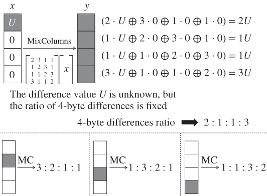
Figure 6.20 Ratio of 4-byte differences in a column
The same property can be obtained for different input active byte positions.
6.4.2.3 Collecting Pairs
The attacker obtains a pair of plaintext and ciphertext denoted by ![]() . While the same plaintext
. While the same plaintext ![]() is processed, the attacker injects a fault in the known and fixed byte position at the beginning of round 7 to obtain the faulty ciphertext
is processed, the attacker injects a fault in the known and fixed byte position at the beginning of round 7 to obtain the faulty ciphertext ![]() . In Figure 6.19, this position is fixed to the byte position 6. The same procedure is iterated 10 times to collect
. In Figure 6.19, this position is fixed to the byte position 6. The same procedure is iterated 10 times to collect ![]() . In the end, the attacker obtains 10 pairs of correct and faulty ciphertexts that follow the differential propagation in Figure 6.19.
. In the end, the attacker obtains 10 pairs of correct and faulty ciphertexts that follow the differential propagation in Figure 6.19.
6.4.2.4 Key Recovery Procedure
The attacker guesses 4 bytes of the last subkey ![]() and 1 byte of the converted subkey
and 1 byte of the converted subkey ![]() to perform the partial decryption from ciphertext to any 1 byte of
to perform the partial decryption from ciphertext to any 1 byte of ![]() . Figure 6.21 describes the partial decryption from ciphertext to 1 byte of
. Figure 6.21 describes the partial decryption from ciphertext to 1 byte of ![]() and 1 byte of
and 1 byte of ![]() . Note that the order of
. Note that the order of ![]() and
and ![]() operations is exchanged in round 9.
operations is exchanged in round 9.

Figure 6.21 Independent partial decryption with 5-byte guess
From the analysis of the differential ratio, ![]() holds as long as the fault is injected at
holds as long as the fault is injected at ![]() or the other 3 bytes in the same inverse diagonal, that is,
or the other 3 bytes in the same inverse diagonal, that is, ![]() ,
, ![]() and
and ![]() . Hereafter, the attacker aims to compute
. Hereafter, the attacker aims to compute ![]() and
and ![]() independently. As shown in Figure 6.21, subkeys guessed in the partial decryption for
independently. As shown in Figure 6.21, subkeys guessed in the partial decryption for ![]() and for
and for ![]() do not have any overlap. Thus, subkey guesses and partial decryptions can be performed independently.
do not have any overlap. Thus, subkey guesses and partial decryptions can be performed independently.
- The computation for
 requires 5-byte subkey guess,
  and
and  . The guessed bytes are marked by filled circles in Figure 6.21. For each
  possibilities of the 5 subkey bytes, compute
  for all the 10 pairs of
  , where
  . Store the sequence of 10 bytes (
 for 10 pairs) in a list
  . Then, sort the list
  .
. - The computation for
 requires 5-byte subkey guess,
  and
and  . The guessed bytes are marked by bold line in Figure 6.21. For each
  possibilities of the 5 subkey bytes, compute
  for all the 10 pairs of
  , where
  . Store the sequence of 10 bytes (
 for 10 pairs) in a list
  . Then, sort the list
  .
. - Find the match of 10-byte elements in
 and
and  .
.
The attack procedure is also illustrated in Figure 6.22.

Figure 6.22 Key recovery procedure of MitM DFA
6.4.2.5 Evaluation
Step 1 generates 8-bit value of ![]() for 10 pairs, which yields 80-bit sequences to match. After the exhaustive guess of 5 subkey bytes,
for 10 pairs, which yields 80-bit sequences to match. After the exhaustive guess of 5 subkey bytes, ![]() 80-bit sequences are stored in
80-bit sequences are stored in ![]() . Similarly after step 2,
. Similarly after step 2, ![]() 80-bit sequences are stored in
80-bit sequences are stored in ![]() . In step 3,
. In step 3, ![]() pairs are examined for matching 80-bit values. Only one value is expected to match. Thus, the correct 10 subkey bytes are recovered.
pairs are examined for matching 80-bit values. Only one value is expected to match. Thus, the correct 10 subkey bytes are recovered.
By iterating the same attack procedure for different columns, the remaining 8 subkey bytes of ![]() can be recovered. Thus, all the subkey bytes in
can be recovered. Thus, all the subkey bytes in ![]() are recovered.
are recovered.
The data complexity of this attack is 20 chosen plaintexts. It requires 10 fault injections. In step 1, the computational cost is ![]() AES round functions, which is equivalent to
AES round functions, which is equivalent to ![]() AES computations. The memory requirement is storing
AES computations. The memory requirement is storing ![]() 80-bit sequence along with 5 subkey bytes, which is less than
80-bit sequence along with 5 subkey bytes, which is less than ![]() 16-byte values, thus less than
16-byte values, thus less than ![]() AES states. In summary, the attack complexity of the MitM DFA in this fault model is as follows:
AES states. In summary, the attack complexity of the MitM DFA in this fault model is as follows:
6.4.2.6 MitM DFA with Unknown Faulty Byte Position
The feasibility of the attack with unknown faulty byte position depends on the assumption whether the unknown faulty byte position at the beginning of round 7 can be fixed or not.
If the faulty byte position can be fixed (but unknown), what the attacker needs is guessing the diagonal position with the faulty byte. The guess is chosen from at most four patterns. Thus, the computational cost of the attack becomes ![]() rather than
rather than ![]() , but it is still feasible.
, but it is still feasible.
If the faulty byte position cannot be fixed, there is no method to efficiently match the 80-bit sequences. Thus, the attack can no longer recover the key.
Further Reading
- Derbez P, Fouque P and Leresteux D 2011 Meet-in-the-middle and impossible differential fault analysis on AES In Cryptographic Hardware and Embedded Systems - CHES 2011 - 13th International Workshop, Nara, Japan, September 28 - October 1, 2011. Proceedings (ed. Preneel B and Takagi T), vol. 6917 of Lecture Notes in Computer Science, pp. 274–291. Springer-Verlag.
- Kim CH 2011 Efficient methods for exploiting faults induced at AES middle rounds Cryptology ePrint Archive, Report 2011/349. International Association for Cryptologic Research.
- Mukhopadhyay D 2009 An improved fault based attack of the advanced encryption standard In Progress in Cryptology - AFRICACRYPT 2009, Second International Conference on Cryptology in Africa, Gammarth, Tunisia, June 21-25, 2009. Proceedings (ed. Preneel B), vol. 5580 of Lecture Notes in Computer Science, pp. 421–434. Springer-Verlag.
- Phan RC and Yen S 2006 Amplifying side-channel attacks with techniques from block cipher cryptanalysis In Smart Card Research and Advanced Applications, 7th IFIP WG 8.8/11.2 International Conference, CARDIS 2006, Tarragona, Spain, April 19-21, 2006, Proceedings (ed. Domingo-Ferrer J, Posegga J and Schreckling D), vol. 3928 of Lecture Notes in Computer Science, pp. 135–150. Springer-Verlag.
- Piret G and Quisquater J 2003 A differential fault attack technique against SPN structures, with application to the AES and KHAZAD In Cryptographic Hardware and Embedded Systems - CHES 2003, 5th International Workshop, Cologne, Germany, September 8-10, 2003, Proceedings (ed. Walter CD, Koç ÇK and Paar C), vol. 2779 of Lecture Notes in Computer Science, pp. 77–88. Springer-Verlag.
- Sasaki Y, Li Y, Sakamoto H and Sakiyama K 2013 Coupon collector's problem for fault analysis against AES - high tolerance for noisy fault injections In Financial Cryptography and Data Security - 17th International Conference, FC 2013, Okinawa, Japan, April 1-5, 2013, Revised Selected Papers (ed. Sadeghi A), vol. 7859 of Lecture Notes in Computer Science, pp. 213–220. Springer-Verlag.
- Tunstall M, Mukhopadhyay D and Ali S 2011 Differential fault analysis of the advanced encryption standard using a single fault In Information Security Theory and Practice. Security and Privacy of Mobile Devices in Wireless Communication - 5th IFIP WG 11.2 International Workshop, WISTP 2011, Heraklion, Crete, Greece, June 1-3, 2011. Proceedings (ed. Ardagna CA and Zhou J), vol. 6633 of Lecture Notes in Computer Science, pp. 224–233. Springer-Verlag.