
Chapter 5
Side-Channel Analysis and Fault Analysis on Block Ciphers
5.1 Introduction
In this chapter, side-channel analysis and fault analysis on block ciphers are introduced. They belong to the physical attacks or the implementation attacks, in which the attackers attempt to recover the secret information from a cryptographic algorithm implemented in a physical device. A straightforward implementation of the block ciphers can be easily broken by physical attacks without leaving any attack evidence.
In cryptanalysis, it is assumed that the intermediate values, that is, the intermediate calculation result during the cryptographic operation is unavailable to the attackers. In contrast, in the physical attacks, the attackers can obtain information such as the Hamming weight (HW) of an intermediate value by physically manipulating and observing the device. Such information enables the attackers to efficiently recover the secret key of a block cipher.
5.1.1 Intrusion Degree of Physical Attacks
The category of the physical attacks is shown in Figure 5.1. According to the physical intrusion degree to the target device, the physical attacks are sorted into three categories; invasive, semi-invasive, and noninvasive attacks. Generally speaking, the higher the intrusion degree is, the more powerful the attack becomes. However, a deep intrusion is likely to link to a high cost in implementing the attack and may result in leaving much evidence of the performed attacks.

Figure 5.1 Category of physical attacks
Figure 5.2 shows a general structure of an IC chip. Inside the package of the IC chip, the silicon die, on which the gates, wires, memory, and so on are fabricated, is in the center. The IC chip pins are connected to the silicon die via the bonding wires. Without depackaging the chip, the silicon die cannot be contacted directly. Many physical attacks with a high intrusion degree assume a direct contact with the silicon die, which implies that the package of the IC chip must be removed in the attacks.

Figure 5.2 General structure of IC chip
- Invasive attacks invade the silicon die in the target IC chip by removing the package material using chemicals. Well-known invasive attack is based on an observation of the signals on wires or memory cells using a special instrument such as an electronic microscope. This type of attack is very powerful as the intermediate value in the digital circuit becomes transparent to the attackers. On the other hand, performing this type of attack requires relatively expensive equipment and special expertise. Furthermore, the risk of a permanent damage to the target device is relatively high.
- Semi-invasive attacks still require removing the package to disclose the silicon die. However, different from the invasive attacks, the semi-invasive attacks require no direct electrical contact to the internal wires on the silicon die. Therefore, the possibility of the physical damage of the silicon die is largely reduced compared to the invasive attack.
In the semi-invasive attack, the attackers rather change the intermediate values than observing it directly. For example, it has been reported that a high-energy light or an optical laser beam can be used for altering the value in the memory under the semi-invasive attack scenario. The attack utilizing the alternation of the intermediate value is explained in more details later in this chapter.
- Noninvasive attacks do not require the depackaging step. They only require some contact to the pins of the IC chip. Side-channel analysis and fault analysis are included in this type of attacks.
In side-channel analysis, attackers observe physical information leaked from the target device via the side channel. The attackers analyze the so-called side-channel information that contains sensitive information of the intermediate value of a cryptographic operation. As a result, if the attackers know the relationship between intermediate values and side-channel information in some way, the intermediate value could be disclosed, which often leads to the secret key recovery of a cipher.
On the contrary, fault analysis disturbs a cryptographic operation by intentionally injecting faults during a cryptographic computation in order to extract the secret information. It can be performed without causing any damage to the device if the fault is injected with an illegal clock signal, a voltage fluctuation, an electromagnetic interference, and so on. That is, noninvasive fault analysis differs from the semi-invasive one on how to inject the faults. The noninvasive attacks leave little evidence of the attack, so that the device user does not know the fact that the device has been attacked.
Both of side-channel analysis and fault analysis can be achieved using off-the-shelf equipments and do not require much expertise for the attackers. Therefore, noninvasive attacks are regarded as a serious security issue in practice. Thus, they are treated as the main topics of this chapter.
5.1.2 Passive and Active Noninvasive Physical Attacks
As shown in Figures 5.1 and 5.3, depending on the direction of the physical information that is used for the key recovery, the physical attacks can be divided into two types as the passive attacks and active attacks.
- Passive attacks only observe the physical information leaked from the device to the attackers. The attackers do not affect the calculation of the cryptographic algorithms but only collects the leaked information during those calculations. The noninvasive passive attack is side-channel analysis attack, side-channel attack, or SCA for short.
- Active attacks disturb the calculations of the cryptographic algorithms intentionally, which means that the attackers force some known property of the intermediate values to occur in the target device. The assumption of the active attack implies the alternation of the original calculation of the cryptographic algorithms, which is realized by performing the so-called fault injections. Therefore, these attacks are called fault injection attack, fault analysis attack, fault attack, or FA for short.

Figure 5.3 Passive and active attacks
The passive attack and active attack are different but tightly related to each other. For instance, there is an attack in which the attackers use fault injections to obtain the information leakage from the target device and then apply the key recovery algorithms from side-channel analysis to recover the key. The rest of this chapter mainly focuses on the noninvasive attacks on block ciphers including both the passive and active ones.
5.1.3 Cryptanalysis Compared to Side-Channel Analysis and Fault Analysis
Cryptanalysis introduced in Chapter 4 does not use the information related to the intermediate values during the cryptographic calculations. In contrast, side-channel analysis and fault analysis take advantage of the information about intermediate values. Therefore, they become one of the most powerful and practical threats to cryptographic implementations.
Both side-channel analysis and fault analysis require the attackers to be able to contact the target device. However, cryptanalysis only requires the access to the input and output of the target algorithm. As shown in Figure 5.4, the vulnerability of theoretical cryptanalysis comes from the algorithm of the designed cipher, whereas the vulnerabilities of side-channel analysis and fault analysis largely depend on the implementation techniques of the block cipher. In other words, for different implementations of the same algorithm of a cipher, the applications of side-channel analysis and fault analysis could be different.

Figure 5.4 Cryptanalysis compared to side-channel analysis and fault analysis
5.2 Basics of Side-Channel Analysis
5.2.1 Side Channels of Digital Circuits
The modern cryptographic modules are all based on the digital computation that is performed on physical devices. When executing the computation, the cryptographic device consumes power and causes heat, electromagnetic radiation, and so on. That is, physical manipulation and interaction of the cryptographic device open new information channels available to the attackers. As shown in Figure 5.5, the leakage channels of the physical information are considered side channels in contrast to the main channel that transmits input and output data of a block cipher. When the cryptographic devices are available to the attackers, via the side channels, the side-channel information such as power consumption can be measured during the cryptographic calculation. Because the side-channel information depends on the value of the processed data (intermediate value), the sensitive information that is related to the key could be extracted by analyzing the side-channel information. The analog physical leakage such as the power consumption or the electromagnetic radiation leaked from a device is called side-channel information. Note that the side-channel information such as the power consumption always contains noise that is not related to the cryptographic calculations.

Figure 5.5 Main channel and side channel for block ciphers
The side channels exist for any physical devices. Thus, the security against side-channel analysis cannot be ignored when a cryptographic algorithm is physically implemented. A even well-designed cryptographic algorithm does not ensure its security when it is implemented in a practical device such as CPU (central processing unit) and smart card. Even for the same cryptographic algorithm, many different implementations can be achieved. Minimizing the information leakage via side channels with the least cost is set as one of the goals of the implementations.
5.2.2 Goal of Side-Channel Analysis
The goal of side-channel analysis is twofold. One is for device designers to verify the security of the device and the other is for the attackers to break the cryptosystem. The chip designers attempt to minimize the side-channel information leakage that can be used for the key recovery, in designing their chip. On the other hand, the attackers attempt to find useful side-channel information and the analysis method to maximize the side-channel information leakage. These two perspectives differ slightly depending on whether the secret key is known or not. As mentioned earlier, this chapter mainly stands in the attacker's perceptive, so the key recovery in an unknown key setting is placed as a central discussion item.
When the secret key in a cryptographic device is exposed, the security of the system using the device would be broken. The attackers attempt to recover the secret key of a cipher with the least effort. Therefore, the most vulnerable part of the device is of interest to the attackers. Given a cryptographic device, the attackers explore what kinds of attack could be the most powerful side-channel analysis. First of all, if the attackers can read the value of the secret key directly from the device via a side channel, it will be the most powerful side-channel analysis. However, this cannot be easily done especially with a tamper-proofed device. The secret key is usually stored in nonvolatile memories inside the device that is protected by a package as shown in Figure 5.2. Therefore, it is almost impossible to read out the secret key physically without breaking the package of the chip. This kind of attack cannot be realized with the noninvasive side-channel analysis.
Although the secret key cannot be accessed outside the device, it is used for performing the cryptographic computation when encrypting the plaintext. Accordingly, the intermediate values during the computation are related to the secret key, and the side-channel information contains information correlated to the value of the secret key. As long as the secret key information can be extracted from the side-channel information using side-channel analysis, the key recovery can be achieved.
In order to achieve a successful key recovery, a requirement for side-channel analysis is the knowledge of the target device for the attackers. On the one hand, theknowledge of the target device helps the attackers to understand the relations between the intermediate values and the side-channel information. On the other hand, the attackers attempt to achieve the side-channel analysis that requires the least knowledge of the target device to recover the key. The knowledge of the device includes the information about the architecture of the target cryptographic device and the characteristics of the power consumption of the device.
In addition to the knowledge of the device, the attackers' computational capability is tightly related to the success of the key recovery. When analyzing the side-channel information, the attackers need to reduce the computational cost for the key recovery by dividing it into multiple small computations until the attackers can compute them within a reasonable analysis time. This is called divide-and-conquer technique, which is detailed later in this chapter. The key recovery computation that can be done by personal computers is considered a real threat because every attacker can use a personal computer with a decent computational ability in the current age.
The key recovery algorithm extracts useful information from a set of noisy data. Regarding the required number of traces to successfully recover a key, the smaller the number of traces is, the more advanced the key recovery algorithm is. That is, the number of traces should be minimized for the key recovery of the side-channel analysis, and it is commonly used as an efficiency metric of the key recovery algorithms.
5.2.2.1 Trade-Off in Side-Channel Analysis
In practice, the parameters, that is, the knowledge of the target device, the computational cost, and the required number of traces, to make an efficient side-channel analysis are conflicting with each other. For example, less knowledge of the target device implies that more traces are required for the key recovery. In addition, when the number of traces for the key recovery is limited, a more complicated key recovery algorithm is required with more computational cost. Therefore, the attackers always attempt to find a reasonable trade-off among the required number of traces, the computational cost, and the required knowledge of the target device as shown in Figure 5.6. In the figure, Attack 2 requires fewer traces than Attack 1 but requires more computational cost and more knowledge of the target device. In this way, the attackers explore the trade-offs suitable for the corresponding the attack scenarios. Note that a similar trade-off also exists for fault analysis.

Figure 5.6 Trade-offs in side-channel analysis
5.2.3 General Procedures of Side-Channel Analysis
The general procedures of side-channel analysis can be divided mainly into two steps as shown in Figure 5.7.
- Manipulation of the device for measuring physical information: the attackers should have the access to the device. For example, control the plaintext and/or ciphertext of a block cipher. Then, the attackers need to use side channels to obtain the side-channel information when the device is performing the cryptographic computation. For the passive attack, the attackers only observe or measure the physical information leaked from the device.
- Data analysis of the side-channel information: the side-channel measurement data goes through the data processing such as data alignment and noise reduction. If the side-channel information includes enough information regarding the secret key, and the attackers have an ability to extract key-related information from the data, the key recovery attack will be successful. In this regard, it is natural that the attackers attempt to obtain more traces and find more powerful analysis tools in order to achieve an efficient key recovery attack.

Figure 5.7 General procedures of side-channel analysis
5.2.4 Profiling versus Non-profiling Side-Channel Analysis
According to the attackers' ability, side-channel analysis can be divided into profiling analysis and non-profiling analysis. The challenges of side-channel analysis are based on how to link the side-channel leakage to the intermediate values and how to reduce the noise of the side-channel measurement data to identify the correct key. Profiling analysis and nonprofiling analysis differ in the methods for linking the side-channel leakage to intermediate value.
For profiling analysis, the attackers can use a profiling device, which has similar characteristics of the side-channel leakage of the target device with a configurable key, to learn the details of the leakage characteristics of the target device. The profiling device could be the same manufacture as the target device, so that the similar leakage characteristics can be expected. Figure 5.8 shows the basic idea of a profiling side-channel analysis. Profiling analysis has two phases; the profiling phase and the attack phase. In the profiling phase, the attackers study the unique leakage characteristics of the target device using the profiling device with a configured key. Note that as the attackers do not know the key, K, in the target device, the configured key, ![]() , is different from K as shown in Figure 5.8. Thus, the attackers attempt to consider how to make the leakage profile that does not largely depend on the value of key. The leakage characteristics learned from the profiling device are called a leakage profile. In the attack phase, the attackers attempt to recover the unknown key in the target device with the help of the leakage profile. Profiling analysis requires fewer traces in the attack phase compared to the nonprofiling analysis.
, is different from K as shown in Figure 5.8. Thus, the attackers attempt to consider how to make the leakage profile that does not largely depend on the value of key. The leakage characteristics learned from the profiling device are called a leakage profile. In the attack phase, the attackers attempt to recover the unknown key in the target device with the help of the leakage profile. Profiling analysis requires fewer traces in the attack phase compared to the nonprofiling analysis.

Figure 5.8 Profiling side-channel analysis
For nonprofiling analysis, the attackers attempt to use general knowledge of the target device to construct a leakage model (LM) that describes the relations between processed data and the side-channel information in the key recovery based on the knowledge of the target device. With the LM and the side-channel measurement data obtained from the target device, nonprofiling analysis conducts the key recovery in the attack phase. Figure 5.9 shows the basic idea of nonprofiling side-channel analysis. More details of nonprofiling side-channel analysis are explained later with the attack examples.

Figure 5.9 Nonprofiling side-channel analysis
5.2.5 Divide-and-Conquer Algorithm
Divide-and-conquer algorithm is the essence to explain the effectiveness of side-channel analysis. The information leakage via the side channels is accompanied by noise in the traces. Therefore, in the sense of the signal quality, the side-channel information is significantly worse than the digital information such as plaintexts and ciphertexts. However, the fact that the side-channel leakage can be linked to the intermediate value makes side-channel analysis very powerful.
Side-channel analysis only focuses on a part of the cryptographic algorithm that is close to the public data, that is, plaintexts or ciphertexts. For a part of the cryptographic algorithm, in most cases, it is easy and obvious to divide the computation into small ones. For example, the related key bits for a small part of the attacked algorithm can be 32 bits, 8 bits, or even 1 bit. To achieve both the security and the efficiency, modern block ciphers are tend to be composed of many small components. For a part of the algorithm that is focused by side-channel analysis, usually it can be broken down into small computational parts. Then, the key piece used for each part can be exhaustively tested with a reasonable computational cost. The side-channel information can be used in the exhaustively test to recover each small piece of the key.
Figure 5.10 shows the concept of a divide-and-conquer algorithm. The recovery of a 128-bit key is divided into the recovery of sixteen 8-bit key pieces. After recovering and combining all the 8-bit key pieces, the original 128-bit key can be recovered.
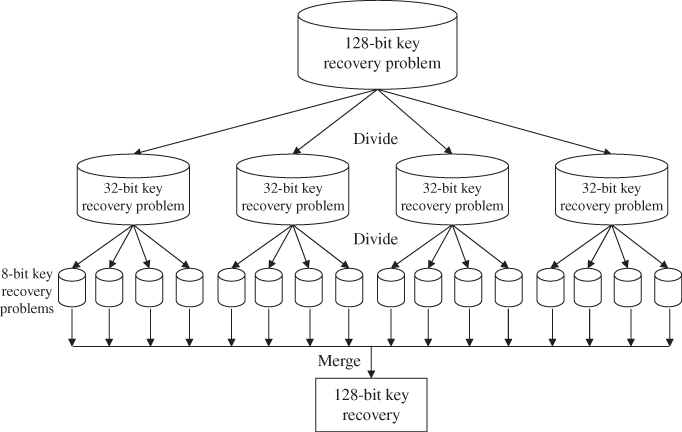
Figure 5.10 Concept of divide-and-conquer algorithm
In side-channel analysis, the key recovery attack for each key piece can be regarded as a brute-force attack with the help of side-channel information. The basic concept of the brute-force attack has been introduced in Chapter 4. For a block cipher such as AES-128, a pair of plaintext and ciphertext can be used to verify the correctness of a guess of the 128-bit key. The guess of the key is used to encrypt the plaintext to get a corresponding ciphertext. Then, the value of the calculated ciphertext is compared with the real one. As long as the calculated ciphertext is different from the real one, it is sure that the current guess of the key is different from the real key.
When the attackers discard the wrong key candidates, the key space can be reduced. If the key space can be continuously reduced, eventually the key recovery is possible for the attackers. However, the brute-force attack for a modern cryptographic algorithm, whose key size is at least 128 bits, cannot be finished practically because there are too many key candidates to be tested even with the fastest super computer in the world.
Instead of using pairs of plaintext and ciphertext in the original brute-force attack, pairs of side-channel leakage and public data, that is, plaintext or ciphertext, are used in the key recovery of side-channel analysis. With the divide-and-conquer algorithm, the key recovery of the full key becomes the recovery of several small key pieces. For each key piece, the number of all possible key candidates is small enough to be exhaustively verified.
Assume that the side-channel leakage can be converted into the exact intermediate values with probability 1. Then, the brute-force attack in side-channel analysis becomes exactly the same with the one introduced in Chapter 4. In practice, the side-channel key recovery algorithms are developed to convert the side-channel leakage to the information of intermediate values.
5.3 Side-Channel Analysis on Block Ciphers
This section introduces the details for side-channel analysis on block ciphers. As the most promising method for side-channel analysis, power analysis is explained. Power analysis receives the most attention in side-channel analysis research area as the power consumption is inevitable for the cryptographic computations and it iseasy to be measured.
In the introduction of power analysis, the measurement of the power traces and the general key recovery algorithm will be explained. Several detailed key recovery algorithms for power analysis and their attack results on two hardware AES implantations will be explained.
5.3.1 Power Consumption Measurement in Power Analysis
In this chapter, side-channel measurement data denotes the sets of digitalized information converted from analog physical leakage at a certain sampling frequency. They contain the digitalized physical leakage against the discrete time determined by the sample points. The side-channel measurement data is also called traces, for example, power traces in the case for measuring the power consumption.
The side-channel measurement data is digitalized information converted from analog physical leakage that is significantly influenced by a measurement setting, environmental parameters, and so on. Thus, in the side-channel measurement data, measurement noise inevitably exists. The noise in the power traces is relatively small compared to other side-channel information. The attackers attempt to improve the measurement setup to reduce the measurement noise in their measurement data.
As shown in Figure 5.11, general-purpose oscilloscopes, probes, and resistors can be used in measuring the power consumption. The oscilloscope samples the voltage fluctuation along the time and records them as a power trace. The target device is usually an IC chip, in which an cryptographic algorithm is implemented.

Figure 5.11 A typical power measurement setup
The power supply and the ground are denoted by VDD and GND in Figure 5.11. For the power consumption measurement, the resistor is inserted between the VDD of the device and the VDD pin of the IC chip or between the GND of the device and the GND pin of the IC chip. The voltage drop by the resistor is related to the power consumption of the cryptographic algorithm, so the attackers use it for the SCAs.
In the measurement of power consumption, a probe is used for transmitting the voltage fluctuation to the oscilloscope. There are mainly two types of probes used for the power consumption measurement; differential probe and passive probe. The differential probe is able to measure the voltage difference between two measurement points. The passive probe can measure the voltage of a measurement point against the ground of the device.
In order to measure the power consumption that is useful for the key recovery, the measurement timing is very important. The power consumption measurement should be performed when the target device is performing a cryptographic algorithm. The appropriate timing for the oscilloscope to sample and record the power consumption can be achieved using a trigger signal. The trigger signal is usually obtained from the target device itself and has a fixed timing relationship with the cryptographic algorithm. Thus, the trigger signal can be used to achieve the alignment of power traces for multiple power measurements. The accuracy of the trigger signal directly relates to the accuracy of the timing alignment for multiple power traces, which could affect the efficiency of power analysis eventually.
The side-channel measurement data or the traces are normally plotted as a continuous line along the time axis or the sample point axis. In accordance with the measurement setup shown in Figure 5.11, an illustration of the measurement data is shown in Figure 5.12. The trigger signal from passive probe 1 detects a start signal of the cryptographic algorithm. The measurement data from differential probe is the sampled voltage difference between point A and point B, which is related to the current of the resistor connected to the VDD pin. The measurement data from passive probe 2 is the sampled voltage at point C, which is related to the current flowed via the GND pin. In Figure 5.11, the traces from differential probe and from passive probe 2 are synchronized by the same trigger signal. Thus, these two traces should contain the almost same information about the power consumption of the target IC chip. In practice, both the VDD part and the GND part can be chosen to perform the power measurement.

Figure 5.12 Illustration of observed data for power measurement setup shown in Figure 5.11
An example of the power trace from a real hardware implementation of AES is shown in Figure 5.13. The power trace is a line that connects all the neighboring sampled voltage points. The horizontal axis stands for the time or the sample points. The vertical axis is the voltage of measurement result in an arbitrary unit that is denoted by “a.u.” There are 11 power consumption peaks in Figure 5.13. They correspond to one clock cycle for each of the 10 rounds of AES-128 and one more clock cycle for the data transfer. Note that the public data such as plaintexts and ciphertexts could be recorded by the attackers depending on the attack scenario as well.

Figure 5.13 Power consumption trace example for hardware implementation of AES
Algorithm 5.1 illustrates the procedures of the collection of power traces. For a set of plaintexts ![]() , the corresponding ciphertexts
, the corresponding ciphertexts ![]() and the power traces
and the power traces ![]() are collected. The jth sample point of the ith power trace is denoted by
are collected. The jth sample point of the ith power trace is denoted by ![]() , where
, where ![]() and
and ![]() . Thus, the ith power trace
. Thus, the ith power trace ![]() is represented as a sequence set of M sampling points, that is,
is represented as a sequence set of M sampling points, that is,
Figure 5.14 shows the illustration of the data measurement of the plaintexts/ciphertexts and the power traces.

Figure 5.14 Data measurement of power analysis
In the measurement data of power traces, the attackers expect that they contain the side-channel information leakage or side-channel leakage that is the useful information for the key recovery. The power consumption of a cryptographic device could contain the information about the intermediate value. As the intermediate value could be related to the secret key, the attackers may be able to use some key recovery algorithms to extract the side-channel information leakage inside the side-channel measurement data.
5.3.2 Simple Power Analysis and Differential Power Analysis
The key recovery algorithm of power analysis can be mainly divided into two types as simple power analysis (SPA) and differential power analysis (DPA), which were proposed in Kocher et al. (1999). SPA uses only one single power trace or the mean of a few power traces to perform the key recovery. Assume that there are N power traces, each has M sample points. The mean of these power traces can be represented by

In SPA, the value of the secret key can be understood only by reading the shape of the power trace.
The scenarios of successful applications of SPA are limited. One of successful applications of SPA is the modular exponentiation of the RSA (Rivest–Shamir–Adleman) algorithm that is a widely used public key cryptographic algorithm. Comparing the power trace with the power consumption patterns, the key recovery of SPA can be performed. Figure 5.15 shows an attack illustration of SPA where the power consumption patterns for value 1 or 0 of each bit of the secret key can be easily identified. As SPA on AES implementation is hardly possible, this chapter skips more details of SPA.

Figure 5.15 Attack illustration of simple power analysis
In contrast to SPA, DPA refers to power analysis that performs statistical analysis on multiple traces in the key recovery. For DPA, the secret information cannot be directly retrieved with one or a few power traces. A large amount of power traces are normally required to perform statistical analysis that can extract a small difference among the power traces. In practice, the number of the power traces used for DPA ranges from hundreds to a few millions. Hereafter, this chapter mainly focuses on the key recovery algorithm of the DPA attacks.
5.3.3 General Key Recovery Algorithm for DPA
This section explains the general key recovery algorithm for the DPA attacks. The input for the key recovery algorithm includes the power traces and the public data such as ciphertexts. The goal of the key recovery algorithm is to obtain the secret key, which is achieved by making sure that the correct secret key value can be distinguished from others. The attackers construct links among the secret key, the public data, and the side-channel measurement data to achieve the successful key recovery.
As the attackers do not know the value of the secret key, DPA starts from guessing the value of the key as a key guess. Then, the attackers use the links among the key, the public data, and the power traces to perform some calculations using the current key guess. For every possible key guess, the above-mentioned calculation is performed.
The attackers know that only if the key guess is correct, the links between the key guess and the measurement data can be established and a meaningful result can be obtained. For the wrong key guesses, the above-mentioned calculation behaves with no reasons; some meaningless results will be obtained. Therefore, it is expected that the calculation result for the correct key guess can be distinguished from those for the wrong key guesses. In other words, from the calculation results corresponding to all key candidates, the attackers can identify the correct key.
In a general key recovery algorithm with DPA, the links among the key, the public data, and the power traces can be broken down into selection function (SF), LM, and evaluation function (EF). A brief explanation is given as follows.
- Selection function is a link from the key guess and the public data to an intermediate value called target intermediate value, I. The SF is normally a part of the cryptographic algorithm that calculates the target intermediate value using the public data and a key guess, G. For example, when attacking AES using the ciphertexts as the public data, the SF could be a partial decryption using the last round of AES.
- Leakage model is a link from the target intermediate value to the rough estimation of the power consumption, T. The LM roughly describes the relations between intermediate values and the side-channel information. In the key recovery algorithms, an LM is a function that maps the calculated target intermediate value to some values that represent rough characteristics of the power consumption. For example, the attackers use the results of the LM with a certain key guess to classify the power traces into different groups and expect that the power traces in different groups have different power consumptions. Note that the LM does not have to describe real power consumption very accurately. As far as the rough leakage characteristics described by the LM match the real power consumption, the key recovery of DPA is possible with enough power traces.
- Evaluation function is a link from the rough estimation of power consumption and the real power traces to the credibility of the key guess. Evaluation function uses a statistical tool to extract the relations between the rough estimation of power consumption and the real power traces. The extracted relations are quantitatively expressed as a value that can represent the credibility of the current key guess. In the key recovery algorithm, the EF maps the rough estimation of power consumption with a key guess and the real power traces to the credibility of the current key guess. Finally, the credibilities of all key candidates are compared with each other, and the one that is most likely to be the correct key is picked up as the attack result.
Figure 5.16 shows an illustration of the general key recovery algorithms for DPA. The key guess is linked to the target intermediate value using public data and an SF. The target intermediate value is linked to the rough estimation of power consumption using an LM. The rough estimation of power consumption is linked to the credibility of the current key guess using the real power traces and an EF. Finally, the DPA attack returns the key guess that is most likely to be the correct key.
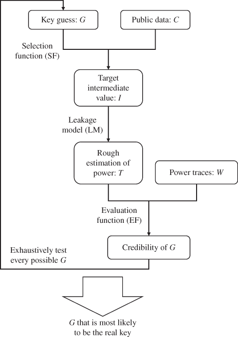
Figure 5.16 General key recovery algorithms for differential power analysis
The key recovery algorithm of DPA is shown in Algorithm 5.2. In Algorithm 5.2, the ciphertexts are used as the public data and only a specific single sample point, j, of the power traces is used. Step 1 in Algorithm 5.2 is the exhaustive search for all the possible key candidates. Step 3 is the SF and the LM calculation using the ciphertexts and key guess as the inputs. The calculation result of step 3 denoted by T is expected to have some relations with the real power consumption when the key guess is correct. Step 5 uses the EF to extract the relations between T and the power traces, and its result denoted by ![]() is obtained for every key candidates as their credibilities as a real key. Finally, step 7 picks up the G that is most likely to be the expected result for the correct key as the attack result.
is obtained for every key candidates as their credibilities as a real key. Finally, step 7 picks up the G that is most likely to be the expected result for the correct key as the attack result.
In practice, the attackers are not sure about which of the sample points is the most useful one in the key recovery. The natural solution is to repeat Algorithm 5.2 for each sample point of the power traces. Then based on the results of all the sample points, the key recovery is performed. Note that step 3 in Algorithm 5.2 does notneed to be repeated when attacking different sample points. Thus, the key recovery algorithm with all the sample points in the traces examined can be performed as shown in Algorithm 5.3.
Step 5 in Algorithm 5.2 is extended to steps 5 to 7 in Algorithm 5.3. The evaluation result in Algorithm 5.2 for each key guess is in the form of 1 value. The evaluation result in Algorithm 5.3 for each key guess is in the form of a trace that has M values as shown in step 8 in Algorithm 5.3. The other parts of Algorithms 5.2 and 5.3 are exactly the same.
Hereafter, for the key recovery algorithm of each specific attack method, all the sample points will be used to demonstrate the attack result for the entire AES calculation. In practice, the attackers can pick a few sample points to perform the DPA attacks such that the computational cost can be reduced.
5.3.3.1 How to Construct SF
The construction of an SF is essentially the same as the selection of the target intermediate value. When the target intermediate value is fixed, the SF is the calculation between public data to the intermediate value following the specification of the block cipher.
To make the key recovery in DPA possible, the target intermediate value must be related to both the power measurement data and the key guesses. If the target intermediate value is not related to the measurement data, the link to the real power traces cannot be established. Thus, the key recovery will fail. If the target intermediate value is not related to the secret key, for example, using the ciphertext as the target intermediate value, the calculated credibilities will become the same for all the key candidates. Thus, the key recovery will fail as well.
To make the DPA attack efficient, the selection of the target intermediate value should have the following two features.
- A small key piece, for example, a key byte, is involved in the SF, so that the divide-and-conquer algorithm is applied with a reasonable computational cost. To achieve this, the target intermediate value should be close to the public data in the cryptographic algorithm, for example, one round or two rounds before the ciphertext.
- The target intermediate values calculated with a wrong key guess can be treated to be independent of the real ones. When the key guess is correct, all the calculated target intermediate values are the same with the real ones. As long as the leakage function and the EF are reasonable, the link between the rough estimation of power consumption and the real traces can lead to a high credibility for the correct key. For the wrong key guess, if there is no dependency from the wrong target interminable values to the real ones, the calculated credibility for the wrong key guesses can be treated as meaningless values and the key recovery becomes possible. In order to achieve the independence between wrong target intermediate values and the real ones, the SF should involve some nonlinear calculations, such as the
 operation of AES.
When attacking AES, the mostly used target intermediate value is 1 byte of the last round input, that is, ![]() , where B denotes the byte position as
, where B denotes the byte position as ![]() .
. ![]() is the input to the
is the input to the ![]() operation that is an important information source of physical leakage. In addition,
operation that is an important information source of physical leakage. In addition, ![]() is usually stored and updated in DFFs (delay flip flops), which is another important information source of physical leakage. The public data, C and
is usually stored and updated in DFFs (delay flip flops), which is another important information source of physical leakage. The public data, C and ![]() , has the following relation:
, has the following relation: ![]() . When
. When ![]() , the first byte of
, the first byte of ![]() can be calculated as
can be calculated as ![]() involving 1 byte of the secret key and the nonlinear S-box calculation. Hereafter, for the DPA attacks on AES,
involving 1 byte of the secret key and the nonlinear S-box calculation. Hereafter, for the DPA attacks on AES, ![]() is used as the target intermediate value and
is used as the target intermediate value and ![]() is the key byte to recover.
is the key byte to recover.
5.3.3.2 How to Construct LM
The LM roughly describes the relations between intermediate values and the side-channel information. This section explains three LMs that are based on simple assumptions about the power consumption. These three LMs will be applied to the attacks examples as shown later in this chapter.
- Single-bit model
The most straightforward assumption to construct an LM is that processing different intermediate values leads to different power consumptions. If the attackers only focus on 1-bit value of the intermediate value, the power consumptions are different when this 1-bit value is 1 or 0. Hereafter, this LM is called the single-bit model. For a CMOS (complementary metal oxide semiconductor) circuit, the motivation of considering the single-bit model is due to the fact that value 1 requires the charge of electrons to a capacitor, whereas the value 0 leads to discharge of electrons.
- Hamming weight (HW) model
The single-bit model can be extended to the HW model, where the values of multiple bits are considered. In the single-bit model, it is assumed that processing value 1 and processing value 0 have different power consumptions. In the HW model, it is assumed that all the bits of a multiple-bit intermediate value follow the single-bit model. That is, the power consumption of a multiple-bit intermediate value is proportional to the number of 1s in it. The number of 1s in a value is called HW. Therefore, this LM is called HW model. Following the HW model, for an intermediate value
31, one can use HW(31) = 3 to roughly estimate the power consumption. - Hamming distance (HD) model
The HW model focuses on the intermediate value at a specific timing. For the HD model, the update of intermediate values from one state to another state is the focus. For each bit of an intermediate value, switching the value of this 1-bit intermediate value and keeping the value of this 1-bit intermediate value could have different power consumptions. In a CMOS circuit, the value switch requires either charge or discharge of a capacitor, while keeping the same value does not. On the basis of this assumption, as a very rough LM, the power consumption is expected to be proportional to the number of bit-flips of two states of an intermediate value. The number of bit-flips between two values is called HD. Therefore, this LM is called HD model. Following the HD model, for an intermediate value changing from
31to83, one can use HD(31,83) = HW(31
83) = 4 to roughly estimate the power consumption.
5.3.3.3 How to Construct EF
The EF is some statistical tool to extract the relationship between the rough estimation of the power consumption and the real ones. Thus, the selection of the EF is largely related to the description of the LM. For example, when a high correlation is expected between the rough estimation of the power consumption and the real power traces, the correlation coefficient calculation can be used as an EF. The construction of the EF is explained in details for each attack algorithm.
5.3.4 Overview of Attack Targets
This section briefly explains the implementations of two hardware AES implementations named AES-pprm1 and AES-comp, which were proposed in Morioka and Satoh (2002) and Satoh et al. (2001). Both AES-pprm1 and AES-comp are without any countermeasures against side-channel analysis. Later, the power traces corresponding to these two hardware implementations of AES are used to demonstrate the detailed power analysis algorithms.
5.3.4.1 Hardware Implementation of AES-pprm1 and AES-comp
The implementations of AES-pprm1 and AES-comp share the same basic architecture, that is, a parallel implementation using the loop architecture. Each AES round is calculated inside 1 clock cycle. In the performed key recovery algorithms later in this chapter, only the last round of AES is analyzed, which has the ![]() ,
, ![]() , and
, and ![]() operations. For the
operations. For the ![]() operation, there are 16 S-box circuits in the combinatorial logic and they are calculated in parallel. The
operation, there are 16 S-box circuits in the combinatorial logic and they are calculated in parallel. The ![]() operation is implemented by arranging the wires in the circuit. The
operation is implemented by arranging the wires in the circuit. The ![]() operation is the XORs with the subkey
operation is the XORs with the subkey ![]() . The illustration of the hardware architecture of the last round for AES-pprm1 and AES-comp is shown in Figure 5.17.
. The illustration of the hardware architecture of the last round for AES-pprm1 and AES-comp is shown in Figure 5.17.

Figure 5.17 Hardware architecture of last round of AES-pprm1 and AES-comp
Owing to the fact that 16 S-boxes are calculated in parallel, the measured power consumption can be considered the summation of the power consumption of all the 16 S-boxes. As mentioned earlier, in the key recovery of AES, the key bytes are recovered byte by byte. The target intermediate value is set to 1 byte of value that is related to 1 byte of the key. Thus, it is favorable for the attackers to measure the power consumption for each S-box independently. However, for AES-pprm1 and AES-comp the power consumption is measured as the summation of that for each S-box. When targeting one S-box, the power consumption of the other 15 S-boxes can be treated as noise in the key recovery. To understand this, recall that the rough estimation of power consumption is related to only 1 byte of the last AES round input. However, the power traces correspond to the summation of power consumption for 16 bytes of the last AES round input. The power consumption of the other 15 S-boxes makes the relations between the rough estimation and the power consumed by the target byte more difficult to extract.
Here, different from the measurement noise, another type of noise called the algorithmic noise is introduced. The algorithmic noise is caused in the key recovery algorithm of side-channel analysis. For a cryptographic device, the measured side-channel traces could correspond to the information of a lot of signal transitions that occur at the same time. In side-channel analysis, the attackers cannot use all the related signal transitions in the key recovery owing to the limitation of the attacker's computational capability and knowledge of the device. Thus, only a part of the signal transitions is related to a specific attack following the divide-and-conquer approach. Simply speaking, the attack algorithm attempts to recover the key piece by piece, but the data measurement cannot measure the side-channel information for each piece independently. Thus, the algorithmic noise appears in the attack. The signal transitions that are not related to the current side-channel analysis are considered the algorithmic noise.
Existence of the algorithmic noise depends on the target hardware architecture and the key recovery algorithm. Namely, the algorithmic noise is not introduced by the measurement but by the key recovery algorithm.
5.3.4.2 S-Box Implementation of AES-pprm1 and AES-comp
The difference between AES-pprm1 and AES-comp is the implementation methods of their S-boxes. The S-box for AES-pprm1 is implemented using the 1 stage Positive Polarity Reed-Muller. As shown in Figure 5.18, the S-box of AES-pprm1 has a special structure that is an AND gate array followed by an XOR gate array. In the AND gate array and the XOR gate array, only the AND gates or the XOR gates are used. AES-pprm1 is used as an experimental implementation that is not likely to be used in a practical device. Owing to the structure of AES-pprm1 S-box, the side-channel leakage of AES-pprm1 can be described clearly with the side-channel LMs. This chapter uses AES-pprm1 to demonstrate the effectiveness of the introduced key recovery algorithms.

Figure 5.18 Hardware architecture of AES-pprm1 S-box
The S-box for AES-comp is implemented in composite-field arithmetic as shown in Figure 5.19. The AES S-box is constructed by two operations mathematically. The first one is the multiplicative inverse for the S-box input, and the second operation is an affine transformation. As introduced in Chapter 1, the multiplicative inverse in S-box is based on modular multiplicative inversion in ![]() . In AES-comp, the multiplicative inverse is separated into three steps. In the first step, the S-box input is converted from its original field into the composite field by an isomorphism function
. In AES-comp, the multiplicative inverse is separated into three steps. In the first step, the S-box input is converted from its original field into the composite field by an isomorphism function ![]() . In the second step, the multiplication inverse in the composite-field is calculated. In the third step, the multiplication inverse is converted back to the original field by an inverse isomorphism function
. In the second step, the multiplication inverse in the composite-field is calculated. In the third step, the multiplication inverse is converted back to the original field by an inverse isomorphism function ![]() . The purpose of performing the multiplication inverse in the composite field is to achieve an S-box implementation with fewer gates and lower power consumption. AES-comp implementation is widely used in practical devices. Compared to AES-pprm1, it is more difficult to use an LM to match the power consumption characteristics for AES-comp.
. The purpose of performing the multiplication inverse in the composite field is to achieve an S-box implementation with fewer gates and lower power consumption. AES-comp implementation is widely used in practical devices. Compared to AES-pprm1, it is more difficult to use an LM to match the power consumption characteristics for AES-comp.

Figure 5.19 Hardware architecture of AES-comp S-box
In the following section, some tests are performed to see how the introduced three LMs match the real power consumption of AES-pprm1 and AES-comp. That is to say, with the real power traces and the value of the key and ciphertexts, the power traces are divided into different groups according to the intermediate values and the LM. Then it is checked whether the difference exists statistically for different groups of the power traces. In the following test, ![]() power traces for each implementation are used. Each power trace has
power traces for each implementation are used. Each power trace has ![]() sample points. The last round AES input,
sample points. The last round AES input, ![]() , is the focused intermediate value.
, is the focused intermediate value.
5.3.4.3 How LMs Matches Power Traces of AES-pprm1
This section shows how much the single-bit model, the HW model, and the HD model match the power traces of AES-pprm1.
- Single-bit model and AES-pprm1
For the single-bit model, the most significant bit (MSB) of
 is used for the group separation. The power traces are separated into two groups as the group with MSB of
  and the group with MSB of
  . Then, the mean traces for two groups of the power traces are calculated and plotted in the same figure as shown in Figure 5.20. If the single-bit model matches the real power traces, it is expected that one can see some difference between the mean traces of two groups of data.

Figure 5.20 Two mean traces of AES-pprm1 after group separation using single-bit model
Figure 5.20 shows the mean traces of AES-pprm1 for two groups of power traces either MSB of ![]() or MSB of
or MSB of ![]() . From Figure 5.20, the two mean traces are overlapped with each other as the difference between them is too small. To confirm the details, the difference between two mean traces for AES-pprm1 is calculated and plotted as shown in Figure 5.21. There are two peaks around the last two clock cycles of the difference of mean trace, which is zoomed and shown in Figure 5.22. The above-mentioned result confirms that the power traces separated by the single-bit model do have a small difference in the power consumptions. Only when the difference of means (DoM) is calculated, the difference can be observed.
. From Figure 5.20, the two mean traces are overlapped with each other as the difference between them is too small. To confirm the details, the difference between two mean traces for AES-pprm1 is calculated and plotted as shown in Figure 5.21. There are two peaks around the last two clock cycles of the difference of mean trace, which is zoomed and shown in Figure 5.22. The above-mentioned result confirms that the power traces separated by the single-bit model do have a small difference in the power consumptions. Only when the difference of means (DoM) is calculated, the difference can be observed.

Figure 5.21 Difference between two mean traces of AES-pprm1 using single-bit model

Figure 5.22 Zoomed Figure 5.23 in last 2 clock cycles
- HW model and AES-pprm1
For testing the HW model, a method that is based on solving the system of linear functions is used to get more accurate mean traces for nine groups of data corresponding to nine possible values of the HW. The details of the constructing and solving the linear functions are omitted in this chapter.
Figure 5.23 shows the nine mean traces of AES-pprm1 after the group separation using the HW model. Figures 5.24 and 5.25 show the Figure 5.23 zoomed in the last two clock cycles and Figure 5.23 zoomed in the peak around 1.83 µs (microsecond), respectively. It can be seen that the nine mean traces for the sample points before 1.5 µs show no difference at all as they correspond to the first nine AES rounds that are independent of the last AES round input
 . For the last two clock cycles of AES calculation, the nine mean traces correspond to nine HW values show clear differences. In Figure 5.25, it is labeled and confirmed that a higher HW value always shows a higher result of the power consumption. This result implies that the HW model is generally a good LM when attacking the AES-pprm1 implementation.

Figure 5.23 Nine mean traces of AES-pprm1 after group separation using HW model

Figure 5.24 Zoomed Figure 5.23 in last two clock cycles

Figure 5.25 Zoomed Figure 5.23 around 1.83 µs
Interestingly, it is observed that the power consumptions for ![]() to
to ![]() have an increasing sequence of the difference between two consecutive HWs. For example, the difference between the power consumptions of
have an increasing sequence of the difference between two consecutive HWs. For example, the difference between the power consumptions of ![]() and
and ![]() is much larger than that between the power consumption of
is much larger than that between the power consumption of ![]() and
and ![]() .
.
- HD model and AES-pprm1
Following the same approach, the nine mean traces of AES-pprm1 after the group separation using HD model are shown in Figure 5.26. Figures 5.27 and 5.28 show that Figure 5.26 zoomed in the last two clock cycles and Figure 5.26 zoomed in the peak around 1.83 µs, respectively.

Figure 5.26 Nine mean traces of AES-pprm1 after group separation using HD model

Figure 5.27 Zoomed Figure 5.26 in last two clock cycles

Figure 5.28 Zoomed Figure 5.26 around 1.83 µs
As shown in Figures 5.26 and 5.27, the clear difference between the nine mean traces appears at the last clock cycle. In the last clock cycle, the last AES round input is updated to the ciphertext in DFFs. As labeled and confirmed in Figure 5.28, a higher HD always has a higher power consumption in the mean traces of various HD values for AES-pprm1. This result implies that the HD model is also a good LM when attacking the AES-pprm1 implementation. Interestingly, it is observed that the power consumptions for ![]() to
to ![]() have a decreasing sequence of the difference between two consecutive HWs.
have a decreasing sequence of the difference between two consecutive HWs.
5.3.4.4 How LMs Matches Power Traces of AES-comp
This section shows how much the single-bit model, the HW model, and the HD model match the power traces of AES-pprm1.
- Single-bit model and AES-comp
Following the same approach, two mean traces of AES-comp after the group separation using the value of the MSB of
 are shown in Figure 5.29. Similarly to the result of AES-pprm1, these two mean traces show almost no difference in Figure 5.29. To confirm the details, the difference between these two mean traces is calculated and plotted in Figure 5.30. The DoM zoomed in the last two clock cycles is shown in Figure 5.31, in which the difference peak in the second to the last clock cycle appears.
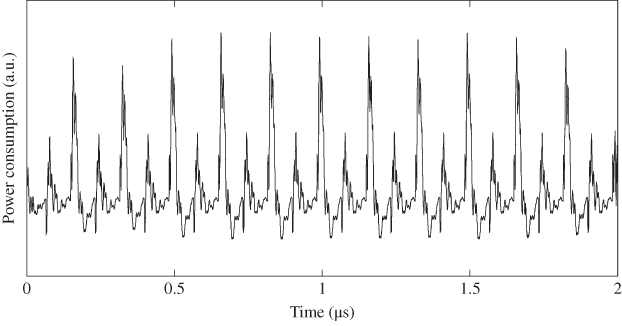
Figure 5.29 Two mean traces of AES-comp after group separation using single-bit model

Figure 5.30 Difference between two mean traces of AES-comp using single-bit model

Figure 5.31 Zoomed Figure 5.23 in last two clock cycles
- HW model and AES-comp
Similar to the AES-pprm1 implementation, the nine mean traces for the AES-comp after the group separation using HW model are shown in Figure 5.32. In the zoomed results as shown in Figures 5.33 and 5.34, it is confirmed that one of the HW values can be distinguished from others. As labeled in Figure 5.34, this distinguishable HW value is corresponding to
 . Thus, the power consumption of AES-comp does not show a clear difference for different HWs of the S-box input except for the case when
  . When the mean traces do not show the clear difference, it implies that the HW model is not a very good LM for AES-comp. However, as
  shows a clear difference from others, power analysis that focuses on the zero value of the HW could be considered, which will be explained in detail later in this chapter. Note that the same pattern of the mean traces can be observed for the second to last clock cycle for AES-comp.

Figure 5.32 Nine mean traces of AES-comp after group separation using HW model

Figure 5.33 Zoomed Figure 5.32 in last two clock cycles

Figure 5.34 Zoomed Figure 5.32 around 1.83 µs
- HD model and AES-comp
Figures 5.35–5.36 show the nine mean traces of AES-comp after the group separation using the HD model. In Figure 5.35, the mean traces for nine HD values show some difference only in the last clock cycle. As labeled and shown in Figure 5.37, in the last clock cycle, one of the nine HD values is largely different from the others. It is confirmed that the most distinguishable mean trace is corresponding to
 . It is also confirmed that in Figure 5.36, the mean traces for
  to
to  show a proportional relationship with the HD value with very small differences. Thus for AES-comp implementation, the HD model could be a good model and the zero-value in HD also leads to a special leakage.

Figure 5.35 Nine mean traces of AES-comp after group separation using HD model

Figure 5.36 Zoomed Figure 5.35 in last two clock cycles

Figure 5.37 Zoomed Figure 5.35 around 1.83 µs
The above-mentioned observations show that in the known key setting, after the group separation according to the LM, the power consumption for different groups does appear some difference. These results imply that the effectiveness of the LM, thus the links among public data, correct key guess, and the power traces can be established. In the attack setting where the key is unknown, the remaining challenge is to see whether or not the credibility for the correct key can be distinguished from the wrong keys. Hereafter, the attack algorithms based on these LMs are explained in detail.
5.3.5 Single-Bit DPA Attack on AES-128 Hardware Implementations
This section explains the DPA attack that is based on the single-bit model, which is called the single-bit DPA attack. The single-bit DPA attack is one of the first introduced SCAs, which can be applied to many devices owing to its very general LM. This section first explains the attack algorithm of the single-bit DPA attack. Then, the AES-pprm1 and AES-comp are used as the attack targets to demonstrate the single-bit DPA attack.
5.3.5.1 SF, LM, and EF for Single-Bit DPA
In single-bit DPA, the attackers focus on only 1 bit of the intermediate value as the target intermediate value. This target intermediate value can be calculated using public data and a guess of a key piece using the SF. The LM in single-bit DPA uses the value of the target intermediate value as the rough estimation of the power consumption, that is, the power consumption is 1 when the target intermediate value is 1 and the power consumption is 0 when the target intermediate value is 0.
The attackers confirm the relations between the rough estimation of power consumptions and the real power traces for each key guess using an EF. Recall that in Figures 5.21 and 5.30, the power consumption difference according to the single-bit model becomes clear when the DoM is calculated for both AES-pprm1 and AES-comp. Similarly, in the single-bit DPA attack, the calculation of DoM is used as the EF.
Specifically, the attackers separate the power traces into two groups according to the value of target intermediate value. Then, the attackers calculate the mean trace for each group of power traces and calculate the difference between two mean traces. This procedure is illustrated in Figure 5.38. For each possible candidate of the small key piece, the group separation and the calculation of DoM are performed.

Figure 5.38 Data processing for each key guess in single-bit DPA
5.3.5.2 Why Key Recovery Could Succeed?
Let us consider the mechanism of the key recovery for single-bit DPA by considering the distributions of intermediate values after the group separation and the calculation of DoM.
- For any intermediate value that is not the target intermediate value, the power consumption that is related to it belongs to the algorithmic noise. As these intermediate values are not used in the group separation, the same distribution of them is expected for each group of power traces. Thus, it is expected that they contribute to an almost zero difference in the trace of DoM.
- For the target intermediate value I, the result of group separation depends on the correctness of the key guess G.
When G is wrong, the attackers expect that the calculated target intermediate values are independent of the real values.1 After the group separation based on the calculated target intermediate values, each group of power traces is expected to have the same distribution of the real values of I. Thus, it is expected that when G is wrong, the target intermediate value contributes to an almost zero difference in the trace of DoM.
When G is correct, all the calculated target intermediate values of I are correct. After the group separation based on the calculated target intermediate values, the power traces in a group either have all the
 traces or all the
  traces. For the target intermediate value, the difference of power consumption for processing
  and processing
  should appear in the trace of DoM. This difference has been confirmed for AES-pprm1 and AES-comp in Section 5.3.4.
As a summary, only when G is correct, the trace of DoM is expected to have some nonzero peaks. Thus, the attackers can identify the trace of DoM that has special nonzero peaks and identify the correct G. With the traces of DoM for all the key guesses, the G that corresponds to the largest absolute value of the DoM, that is, ![]() , should be considered the correct key.
, should be considered the correct key.
Figure 5.39 shows an illustration of the key identification of single-bit DPA. For the correct G, some nonzero peaks are expected in DoM and for wrong key guesses an almost zero difference is expected in DoM. In practice, DoM also shows some nonzero peaks for the wrong key guesses due to two reasons. The first reason is the noise, both the measurement noise and algorithmic noise lead to nonzero values even for wrong key guesses. Another reason is that the target intermediate values forcorrect key and wrong keys are not perfectly independent. The point of DPA is that when enough power traces are used, the effect of the noise is going to be reduced to close to zero and the wrong key guesses will not have a bigger peak than the correct key. Only for the correct key, the group separation is perfect with regard to the value of the target intermediate value.

Figure 5.39 Key identification in single-bit DPA
5.3.5.3 Single-Bit DPA Applied to AES-pprm1 and AES-comp
The single-bit DPA attack is applied to AES-pprm1 and AES-comp targeting ![]() , in which the MSB of
, in which the MSB of ![]() is used as the target intermediate value. The SF includes the
is used as the target intermediate value. The SF includes the ![]() operation, inverse of the
operation, inverse of the ![]() operation, and inverse of the
operation, and inverse of the ![]() operation. The
operation. The ![]() operation can be ignored here as the byte position is not changed for
operation can be ignored here as the byte position is not changed for ![]() .
.
The key recovery algorithm of the single-bit DPA attack targeting ![]() is shown in Algorithm 5.4. In step 3, the MSB of
is shown in Algorithm 5.4. In step 3, the MSB of ![]() is calculated for the group separation of power traces. In steps 5 to 8, the trace of DoM is calculated. The loop in step 1 ensures that the trace of DoM is obtained for each possible key candidate. Step 10 identifies the correct key by finding DoM trace that has the largest nonzero absolute value.
is calculated for the group separation of power traces. In steps 5 to 8, the trace of DoM is calculated. The loop in step 1 ensures that the trace of DoM is obtained for each possible key candidate. Step 10 identifies the correct key by finding DoM trace that has the largest nonzero absolute value.
The attack result of the single-bit DPA attack on AES-pprm1 targeting ![]() is shown in Figures 5.40 and 5.41.2 The traces of DoM for all the 256 key candidates are plotted in Figure 5.40, where “a.u.” stands for arbitrary unit. The black line corresponds to the correct key guess. The area in gray corresponds to the traces of DoM for all the wrong key values.
is shown in Figures 5.40 and 5.41.2 The traces of DoM for all the 256 key candidates are plotted in Figure 5.40, where “a.u.” stands for arbitrary unit. The black line corresponds to the correct key guess. The area in gray corresponds to the traces of DoM for all the wrong key values.

Figure 5.40 Single-bit DPA result targeting  for AES-pprm1
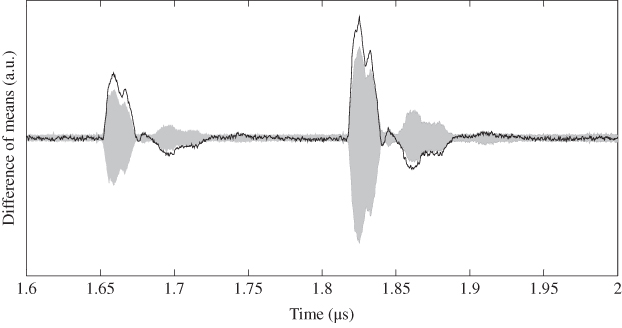
Figure 5.41 Zoomed Figure 5.40 in last two clock cycles
In Figure 5.40, the traces of DoM include the entire AES calculation of 11 clock cycles. As shown in Figure 5.40, the first nine cycles do not help recovering the correct key as the target intermediate value has no relations with the first nine round functions. To make the attack results of the related timing clear, Figure 5.40 zoomed at the last two clock cycles is shown in Figure 5.41. The correct key leads to the highest nonzero value of DoM among all the key candidates. Thus, the key recovery of ![]() is successful for AES-pprm1 using single-bit DPA. There are also some nonzero peaks exist for the wrong key guesses; however, their peaks are smaller than the peak of the correct key guess.
is successful for AES-pprm1 using single-bit DPA. There are also some nonzero peaks exist for the wrong key guesses; however, their peaks are smaller than the peak of the correct key guess.
Similarly, the attack result of the single-bit DPA attack on AES-comp is shown in Figures 5.42 and 5.43. For AES-comp, the black line of the correct key shows the highest absolute value in the traces of DoM at the second to the last clock cycle. However, it is not clear to identify the trace of DoM for the correct key from those results of the wrong key guesses. In this case, the attackers have to either use more power traces to reduce the noise or select a few key candidates with the highest DoM as the attack results.

Figure 5.42 Single-bit DPA result targeting  for AES-comp

Figure 5.43 Zoomed Figure 5.42 in last two clock cycles
The single-bit DPA attack already confirmed the possibility of the key recovery on practical implementations of AES. The same procedure of Algorithm 5.4 can be repeated to recover other key bytes of ![]() . One can also try to find out the least number of power traces to recover all the key bytes. These analyses are related to the attack efficiency, while this chapter mainly focuses on the attack effectiveness. Thus, the details of the full-key recovery are omitted. Hereafter, for each introduced power analysis algorithm, only the key recovery result of
. One can also try to find out the least number of power traces to recover all the key bytes. These analyses are related to the attack efficiency, while this chapter mainly focuses on the attack effectiveness. Thus, the details of the full-key recovery are omitted. Hereafter, for each introduced power analysis algorithm, only the key recovery result of ![]() is demonstrated.
is demonstrated.
5.3.6 Attacks Using HW Model on AES-128 Hardware Implementations
This section explains the DPA attacks using the HW model, which is called the HW-model-based DPA attack in this book. Recall that in single-bit DPA, the SF calculates 1 byte of the last AES round input and uses its MSB as the target intermediate value. The rest 7 bits of the calculated last AES round input are not used in the LM. By effectively extending the single-bit model to a multiple-bit model such as the HW model, the HW-model-based DPA attack can be considered.
For the HW-model-based DPA attack, the target intermediate value is an 8-bit value and the LM is the HW model. The HW model assumes that the power consumption is proportional to the HW of the intermediate value. In other words, the HW model assumes that there is a linear dependency between the HW and the power consumption, which is a correlation between the HW and the power consumption. Following the HW model, the HW of target intermediate values is used as the rough estimation of power consumption. To extract the correlation between the rough estimation of power consumption and the real power traces, the correlation calculation is suitable to be the EF.
For the correlation calculations, the Pearson's correlation coefficient is the most used one. For two data sequences ![]() and
and ![]() , where
, where ![]() , the correlation coefficient can be calculated as
, the correlation coefficient can be calculated as

Assume that the HW model matches the power consumed by the target device. Let us consider the reason that the HW-model-based DPA attack can recover the correct key. When the key guess is correct, the calculated target intermediate values are the real ones. Thus, the calculated HW and the real power traces should lead to a high correlation. When the key guess is wrong, the calculated target intermediate values are expected to be independent of the real ones; thus, the calculated HW has almost zero correlation with the power traces. As a summary, it is expected that the correct key will lead to the peak in the correlations results.
5.3.6.1 HW-Model-Based DPA Attack Applied to AES-pprm1 and AES-comp
For the HW-model-based DPA attack on AES-pprm1 and AES-comp targeting ![]() , the target intermediate value is an 8-bit value as
, the target intermediate value is an 8-bit value as ![]() . For the HW-model-based DPA targeting
. For the HW-model-based DPA targeting ![]() , the key recovery algorithm is shown in Algorithm 5.5. Step 3 is the SF and the LM that uses the HW of
, the key recovery algorithm is shown in Algorithm 5.5. Step 3 is the SF and the LM that uses the HW of ![]() as the rough estimation of the power consumption. Steps 5 to 9 calculate the correlation coefficients between the rough estimation of the power consumption and the real power traces at each sample point. For a key guess G, the correlation coefficients corresponding to all the sample points become a trace of correlation coefficients denoted by
as the rough estimation of the power consumption. Steps 5 to 9 calculate the correlation coefficients between the rough estimation of the power consumption and the real power traces at each sample point. For a key guess G, the correlation coefficients corresponding to all the sample points become a trace of correlation coefficients denoted by ![]() in step 10. Finally, G that leads to the largest value shown in the traces of correlation coefficients is selected as the attack result.
in step 10. Finally, G that leads to the largest value shown in the traces of correlation coefficients is selected as the attack result.
The same power traces of AES-pprm1 and AES-comp are used to demonstrate the attack. The attack result on AES-pprm1 is shown in Figures 5.44 and 5.45. As shown in Figure 5.45, for AES-pprm1, the correct key can be clearly distinguished from others in the last two clock cycles. Compared to the attack result of single-bit DPA, the HW-model-based DPA attack shows an improvement. Recall that the group separation result for AES-pprm1 using HW model as shown in Figure 5.25, the mean traces of the power consumptions have a clear proportional relation against the HW. Thus, the HW-model-based DPA attack has a good attack result against the AES-pprm1.

Figure 5.44 HW-model-based DPA result targeting  for AES-pprm1

Figure 5.45 Zoomed Figure 5.44 in last two clock cycles
The attack result targeting ![]() of AES-comp is shown in Figures 5.46 and 5.47. For AES-comp, the correct key cannot be distinguished from others, which implies a failure in the key recovery. Compared to the attack result of single-bit DPA, the HW-model-based DPA attack shows a worse result. Recall that the group separation result for AES-comp using HW model as shown in Figure 5.34, expect the mean trace for
of AES-comp is shown in Figures 5.46 and 5.47. For AES-comp, the correct key cannot be distinguished from others, which implies a failure in the key recovery. Compared to the attack result of single-bit DPA, the HW-model-based DPA attack shows a worse result. Recall that the group separation result for AES-comp using HW model as shown in Figure 5.34, expect the mean trace for ![]() , the mean traces for
, the mean traces for ![]() to
to ![]() show almost no difference. As the correlation between the rough estimation and the real power traces is too low for the correct key guess, the attack on AES-comp fails.
show almost no difference. As the correlation between the rough estimation and the real power traces is too low for the correct key guess, the attack on AES-comp fails.
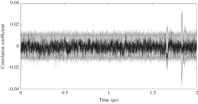
Figure 5.46 HW-model-based DPA result targeting  for AES-comp
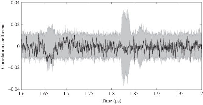
Figure 5.47 Zoomed Figure 5.46 in last two clock cycles
5.3.6.2 Attack Using Zero-Value Model
Recall that as shown in Figure 5.34, the mean trace for ![]() actually shows a difference from the mean traces for
actually shows a difference from the mean traces for ![]() to
to ![]() . Thus, it could be useful to consider an attack that focuses on the zero-value, which is called zero-value analysis. Zero-value analysis takes zero of an 8-bit target intermediate value as a special value for a special side-channel leakage. In the zero-value analysis, the power traces are separated into two groups as the group with zero value and the group with nonzero values. The rest part of the zero-value analysis is the same with the HW-model-based DPA attack.
. Thus, it could be useful to consider an attack that focuses on the zero-value, which is called zero-value analysis. Zero-value analysis takes zero of an 8-bit target intermediate value as a special value for a special side-channel leakage. In the zero-value analysis, the power traces are separated into two groups as the group with zero value and the group with nonzero values. The rest part of the zero-value analysis is the same with the HW-model-based DPA attack.
The reason that the zero value is special for the AES S-box is briefly explained as follows. For AES implementation, most of the side-channel leakage comes from the ![]() operation, which is the only nonlinear operation. AES S-box is constructed by a multiplicative inverse calculation and an affine transformation. However, there is no multiplicative inverse of zero mathematically as any value multiples zero results zero. Thus, AES S-box with its input zero could show a special behavior. For AES S-box, the multiplicative inverse of zero is set to zero instead of being calculated to zero. Thus, for certain implementations such as the AES-comp S-box, the zero input to S-box could lead to a small power consumption as shown in Figure 5.34.
operation, which is the only nonlinear operation. AES S-box is constructed by a multiplicative inverse calculation and an affine transformation. However, there is no multiplicative inverse of zero mathematically as any value multiples zero results zero. Thus, AES S-box with its input zero could show a special behavior. For AES S-box, the multiplicative inverse of zero is set to zero instead of being calculated to zero. Thus, for certain implementations such as the AES-comp S-box, the zero input to S-box could lead to a small power consumption as shown in Figure 5.34.
When targeting ![]() of AES, the target intermediate value is
of AES, the target intermediate value is ![]() , which can be calculated as
, which can be calculated as ![]() . For LM focused on the zero value, the rough estimation of the power consumption is whether the target intermediate value is a zero value. The correlation coefficient is used as the EF to extract the relations between rough estimation of the power consumption and the real power traces. The key recovery algorithm of zero-value analysis is shown in Algorithm 5.6. Note that DoM can also be used to replace the correlation coefficient as there are only two groups for the power separation. The key recovery is expected to be successful if the zero value in the target intermediate value shows a very special leakage.
. For LM focused on the zero value, the rough estimation of the power consumption is whether the target intermediate value is a zero value. The correlation coefficient is used as the EF to extract the relations between rough estimation of the power consumption and the real power traces. The key recovery algorithm of zero-value analysis is shown in Algorithm 5.6. Note that DoM can also be used to replace the correlation coefficient as there are only two groups for the power separation. The key recovery is expected to be successful if the zero value in the target intermediate value shows a very special leakage.
The power data of AES-pprm1 and AES-comp are used to demonstrate the attack result of the zero-value analysis. The attack result on AES-pprm1 is shown in Figures 5.48 and 5.49, in which the correct key byte cannot be distinguished from wrong key values.

Figure 5.48 Zero-value analysis result targeting  for AES-pprm1

Figure 5.49 Zoomed Figure 5.48 in last two clock cycles
The attack result on AES-comp is shown in Figures 5.50 and 5.51. Similarly, the correct key byte cannot be identified. The application of the zero-value attack does not show its advantage over previously introduced attacks.

Figure 5.50 Zero-value analysis result targeting  for on AES-comp

Figure 5.51 Zoomed Figure 5.50 in last two clock cycles
Here, more detailed explanations of the attack result are as follows. First of all, for an 8-bit intermediate value that follows the uniform distribution, the probability of zero occurs with a probability of ![]() or
or ![]() . Therefore, only a small portion of the power traces,
. Therefore, only a small portion of the power traces, ![]() , corresponds to the zero value. This fact increases the difficulty of a zero-value analysis. On the other hand, for AES-pprm1, the zero value of S-box input does not lead to a very special leakage as shown in Figure 5.25. Thus, the key recovery fails. For AES-comp, although
, corresponds to the zero value. This fact increases the difficulty of a zero-value analysis. On the other hand, for AES-pprm1, the zero value of S-box input does not lead to a very special leakage as shown in Figure 5.25. Thus, the key recovery fails. For AES-comp, although ![]() shows a low-power consumption, it cannot overcome the effects of the noise in the performed attack. Actually, by focusing on the second to the last clock cycle in Figure 5.51, the correct key shows a relatively high correlation in the result. It is expected that the correct key can show a distinguishable peak if more traces are used in the attack for AES-comp.
shows a low-power consumption, it cannot overcome the effects of the noise in the performed attack. Actually, by focusing on the second to the last clock cycle in Figure 5.51, the correct key shows a relatively high correlation in the result. It is expected that the correct key can show a distinguishable peak if more traces are used in the attack for AES-comp.
5.3.7 Attacks Using HD Model on AES-128 Hardware Implementations
This section explains the attacks using the HD model on AES-128 hardware implementations called correlation power analysis (CPA). CPA was proposed in Brier et al. (2004). The naming of the attack comes as it is the first proposal for using the correlation coefficient in the EF. Compared to the HW-model-based DPA attack, the only difference of CPA is replacing the HW model by the HD model in the key recovery.
The HW model focuses on the value of an intermediate value at a specific timing, whereas the HD model focuses on the value transitions of an intermediate value. For hardware implementation, the HD model describes the power consumption for the signal transitions in combinatorial logics and the value update for DFFs.
5.3.7.1 CPA Applied to AES-pprm1 and AES-comp
For the CPA attack on AES-128 targeting ![]() , the target intermediate value is still
, the target intermediate value is still ![]() . Then, the HD between the last AES round input and the ciphertext is used as the rough estimation of the power consumption. In the hardware implementation of AES, the last AES round input will be updated to the ciphertext at a specific timing, which is expected to show a correlation with the HD. With a key guess, the target intermediate values and the HD can be calculated as the rough estimation of the power consumption. Then, the correlation calculation, which measures the linear dependence between two variables, is used to extract the relations between the rough estimations and the real power traces. When the key guess is wrong, the calculated target intermediate values are expected to be independent of the real ones. Thus, the calculated HDs are expected to have almost zero correlation with the power measurement data. When thekey guess is correct, the calculated target intermediate values are the real ones. As confirmed in Figures 5.25 and 5.34, the calculated HDs should show a correlation with the real power traces. Therefore, it is expected that the correct key can be identified as it leads to the peaks in the correlations results.
. Then, the HD between the last AES round input and the ciphertext is used as the rough estimation of the power consumption. In the hardware implementation of AES, the last AES round input will be updated to the ciphertext at a specific timing, which is expected to show a correlation with the HD. With a key guess, the target intermediate values and the HD can be calculated as the rough estimation of the power consumption. Then, the correlation calculation, which measures the linear dependence between two variables, is used to extract the relations between the rough estimations and the real power traces. When the key guess is wrong, the calculated target intermediate values are expected to be independent of the real ones. Thus, the calculated HDs are expected to have almost zero correlation with the power measurement data. When thekey guess is correct, the calculated target intermediate values are the real ones. As confirmed in Figures 5.25 and 5.34, the calculated HDs should show a correlation with the real power traces. Therefore, it is expected that the correct key can be identified as it leads to the peaks in the correlations results.
The key recovery algorithm for the CPA attack targeting ![]() is shown in Algorithm 5.7. The only difference between Algorithm 5.7 and Algorithm 5.5 is step 3 of them, specifically the LM. With the calculated
is shown in Algorithm 5.7. The only difference between Algorithm 5.7 and Algorithm 5.5 is step 3 of them, specifically the LM. With the calculated ![]() , the rough estimation of power consumption is calculated as
, the rough estimation of power consumption is calculated as ![]() in Algorithm 5.5 and as
in Algorithm 5.5 and as ![]() in Algorithm 5.7. In steps 5 to 9, the correlation coefficient between the rough estimation and real power traces is calculated at each sample point. For each key guess G, the calculated results become a trace of the correlation coefficients denoted by
in Algorithm 5.7. In steps 5 to 9, the correlation coefficient between the rough estimation and real power traces is calculated at each sample point. For each key guess G, the calculated results become a trace of the correlation coefficients denoted by ![]() . Then in step 12, the attackers observe all the traces of the correlations and identify
. Then in step 12, the attackers observe all the traces of the correlations and identify ![]() as G that shows the largest peak in
as G that shows the largest peak in ![]() .
.
The CPA attack result targeting ![]() of AES-pprm1 is shown in Figures 5.52 and 5.53. As shown in Figure 5.53, the CPA attack can successfully recover
of AES-pprm1 is shown in Figures 5.52 and 5.53. As shown in Figure 5.53, the CPA attack can successfully recover ![]() for AES-pprm1 at the last clock cycle. This result fits the expectation as shown in Figure 5.28; the nine mean traces for different HD distance show clear difference among them. Thus, the HD model is a good attack model to describe the power consumption for AES-pprm1.
for AES-pprm1 at the last clock cycle. This result fits the expectation as shown in Figure 5.28; the nine mean traces for different HD distance show clear difference among them. Thus, the HD model is a good attack model to describe the power consumption for AES-pprm1.

Figure 5.52 CPA result targeting first key byte for AES-pprm1

Figure 5.53 Zoomed Figure 5.52 in last two clock cycles
The CPA attack result targeting ![]() of AES-comp is shown in Figures 5.54 and 5.55. As shown in Figure 5.55, the CPA attack can successfully recover
of AES-comp is shown in Figures 5.54 and 5.55. As shown in Figure 5.55, the CPA attack can successfully recover ![]() for AES-comp as well. For AES-comp, the correlation trace for the correct key is not very clear to be distinguished from others. Recall that as shown in Figure 5.37, the mean trace for
for AES-comp as well. For AES-comp, the correlation trace for the correct key is not very clear to be distinguished from others. Recall that as shown in Figure 5.37, the mean trace for ![]() shows a very low power consumption and the mean traces for
shows a very low power consumption and the mean traces for ![]() to
to ![]() shows a proportional relations with the HD with very small differences. Thus, the leakage related to the HD model for AES-comp is not as much as the AES-pprm1. The attack results confirmed this expectation.
shows a proportional relations with the HD with very small differences. Thus, the leakage related to the HD model for AES-comp is not as much as the AES-pprm1. The attack results confirmed this expectation.

Figure 5.54 CPA result targeting first key byte for AES-comp

Figure 5.55 Zoomed Figure 5.54 in last two clock cycles
5.3.7.2 Attack Using Clockwise Collision Model
As shown in Figure 5.37, the mean trace for ![]() shows a very low power consumption compared to others for AES-comp. Similarly, for AES-pprm1, the mean trace for
shows a very low power consumption compared to others for AES-comp. Similarly, for AES-pprm1, the mean trace for ![]() also shows a relatively low-power consumption as shown in Figure 5.28. Thus, it is reasonable to consider the attack that takes zero value of the HD as a special value, which is called clockwise collision analysis. Clockwise collision refers to the case when an intermediate value has the same value at two consecutive clock cycles.
also shows a relatively low-power consumption as shown in Figure 5.28. Thus, it is reasonable to consider the attack that takes zero value of the HD as a special value, which is called clockwise collision analysis. Clockwise collision refers to the case when an intermediate value has the same value at two consecutive clock cycles.
Owing to the nature of loop architecture, when a byte of the intermediate value has the same value in two clock cycles, there is no toggles in both DFFs and the combinatorial logics. As mentioned in Chapter 2, the stored values at DFFs are the inputs of the combinatorial logics at the beginning of a clock cycle. At the end of a clock cycle, the outputs of the combinatorial logics are stored at DFFs as the evaluation result of combinatorial logics. Consider the case that the DFFs have the same value in two consecutive clock cycles, the inputs of combinatorial logics will have the same value to evaluate in two consecutive clock cycles. In the second clock cycle, the combinatorial logics just keep the state at the end of the first clock cycle and there is no signal transition in the combinatorial logics. Thus, low-power consumption can be expected.
Clockwise collision analysis assumes that the zero value in HD leads to a dominantly special side-channel leakage. Thus, in clockwise collision analysis, the power consumption is separated into two groups according to whether or not the HD is a zero value. The rest part of the attack is the same with zero-value analysis.
For clockwise collision analysis targeting ![]() on AES-pprm1 and AES-comp, the target intermediate value is
on AES-pprm1 and AES-comp, the target intermediate value is ![]() . Whether or not the HD between
. Whether or not the HD between ![]() and
and ![]() is a zero value is used as the rough estimation of power consumption. The correlation coefficient is used as the EF. The key recovery algorithm for clockwise collision analysis targeting
is a zero value is used as the rough estimation of power consumption. The correlation coefficient is used as the EF. The key recovery algorithm for clockwise collision analysis targeting ![]() is shown in Algorithm 5.8. Step 3 in Algorithm 5.8 is the only different part from the attack algorithm for zero-value analysis as Algorithm 5.6.
is shown in Algorithm 5.8. Step 3 in Algorithm 5.8 is the only different part from the attack algorithm for zero-value analysis as Algorithm 5.6.
Algorithm 5.8 is applied to the power traces of AES-pprm1 and AES-comp to show the attack efficiency for the clockwise collision analysis. The attack result on AES-pprm1 is shown in Figures 5.56 and 5.57. For AES-pprm1, the key recovery is successful at the last clock cycle of the AES. Compared to the CPA attack result, the correlation coefficient for key correct key becomes smaller for the clockwise collision analysis. This is because useful information related to ![]() to
to ![]() is ignored in clockwise collision analysis. From the perspective of attackers, the successful key recovery is achieved with a simplified LM.
is ignored in clockwise collision analysis. From the perspective of attackers, the successful key recovery is achieved with a simplified LM.

Figure 5.56 Clockwise collision analysis result targeting  for AES-pprm1

Figure 5.57 Zoomed Figure 5.56 in last two clock cycles
The attack result on AES-comp is shown in Figures 5.58 and 5.59. The successful key recovery has been achieved, and interestingly, the attack result is better than that of the CPA attack. To understand the reason, recall the nine mean traces after the group separation as shown in Figure 5.37. Both CPA and clockwise collision analysis can succeed as they both fit the power consumption of AES-comp. However, as ![]() has a dominate low-power consumption for AES-comp, the simplified LM has a better attack result for AES-comp.
has a dominate low-power consumption for AES-comp, the simplified LM has a better attack result for AES-comp.

Figure 5.58 Clockwise collision analysis result targeting  for AES-comp

Figure 5.59 Zoomed Figure 5.58 in last two clock cycles
5.3.8 Attacks with Collision Model 
This section explains a power analysis that is based on the collision model. In the clockwise collision, the data collision of intermediate values at two clock cycles is considered, for example, the data collision between ![]() and
and ![]() . In the collision model explained in this section, the data collision between two pieces of an intermediate value at the same clock cycle is considered, for example
. In the collision model explained in this section, the data collision between two pieces of an intermediate value at the same clock cycle is considered, for example ![]() and
and ![]() , which was for example discussed in Moradi et al. (2010). The biggest advantage of the attacks with the collision model is that the attackers do not need to assume the LM of target implementation. Recall that the LM describes rough relations between the intermediate value and the side-channel leakage. Instead of LM, the attackers make an assumption that when two pieces of intermediate value have the same value, the corresponding side-channel leakage for them is similar to each other.
, which was for example discussed in Moradi et al. (2010). The biggest advantage of the attacks with the collision model is that the attackers do not need to assume the LM of target implementation. Recall that the LM describes rough relations between the intermediate value and the side-channel leakage. Instead of LM, the attackers make an assumption that when two pieces of intermediate value have the same value, the corresponding side-channel leakage for them is similar to each other.
Figure 5.60 shows the basic principle of the attacks using the collision model for a parallel implementation of AES. The basic assumption is that when two S-box inputs have the same value, that is, ![]() , the side-channel leakage from those two S-boxes are similar to each other, that is,
, the side-channel leakage from those two S-boxes are similar to each other, that is, ![]() . If
. If ![]() ,
, ![]() and
and ![]() . Thus, when the difference between two ciphertext bytes is equal to the difference between the key bytes, the similar leakage of S-boxes can be expected. Therefore, for AES, the attackers can construct a link among the difference of key bytes, the public data, and the case when two S-boxes have similar side-channel leakage. If the attackers can extract the information that two S-boxes have similar side-channel leakage from the power traces, the recovery of the difference between key bytes becomes possible.
. Thus, when the difference between two ciphertext bytes is equal to the difference between the key bytes, the similar leakage of S-boxes can be expected. Therefore, for AES, the attackers can construct a link among the difference of key bytes, the public data, and the case when two S-boxes have similar side-channel leakage. If the attackers can extract the information that two S-boxes have similar side-channel leakage from the power traces, the recovery of the difference between key bytes becomes possible.

Figure 5.60 Principle of data collision inside an intermediate value at last round of AES
There are a few variations of power analysis that use the collision model in the key recovery algorithms. This section only introduces the one that is called correlation-enhanced power analysis collision attack. Hereafter, the attack concept of the correlation-enhanced power analysis collision attack is explained.
In the attack with collision model on AES, with a key guess of ![]() , the target intermediate value of
, the target intermediate value of ![]() can be calculated. As no LM is used in the attacks with collision model, there is no rough estimation of the power consumption mapped from the target intermediate value. However, the power traces can still be separated into groups directly according to the value of the target intermediate value. For an 8-bit target intermediate value, a group separation of 256 groups can be considered. After the group separation, the mean trace of each group can be calculated.
can be calculated. As no LM is used in the attacks with collision model, there is no rough estimation of the power consumption mapped from the target intermediate value. However, the power traces can still be separated into groups directly according to the value of the target intermediate value. For an 8-bit target intermediate value, a group separation of 256 groups can be considered. After the group separation, the mean trace of each group can be calculated.
Note here, for any key guess, the result of the above-mentioned 256 mean traces is exactly the same. Thus, the above-mentioned mean traces after the group separation cannot be directly used to identify the key value, as they are irrelevant to the key value. Actually, the same group separation can be performed without key guess and using the ciphertext directly, as the mapping from ![]() to
to ![]() is bijective. Thus, using
is bijective. Thus, using ![]() directly, the attackers can separate the power traces into 256 groups and calculate the mean trace for each group. Each mean trace is going to correspond to a value of
directly, the attackers can separate the power traces into 256 groups and calculate the mean trace for each group. Each mean trace is going to correspond to a value of ![]() .
.
In the attack with collision model, the goal is set to identify the key byte difference by focusing on two target intermediate values. For example, the attackers focus on recovering ![]() by focusing on
by focusing on ![]() and
and ![]() . For
. For ![]() , the group separation and the calculation of the mean traces can be performed as well. In the group separation for
, the group separation and the calculation of the mean traces can be performed as well. In the group separation for ![]() , each mean trace is going to correspond to a value of
, each mean trace is going to correspond to a value of ![]() . Recall that when
. Recall that when ![]() ,
, ![]() , which means the corresponding mean traces are similar.
, which means the corresponding mean traces are similar.
If the attackers know the value of ![]() , for a mean trace for a value of
, for a mean trace for a value of ![]() , the attackers can find a corresponding value of
, the attackers can find a corresponding value of ![]() such that
such that ![]() and the corresponding mean traces are similar to each other. There are 256 possible values for
and the corresponding mean traces are similar to each other. There are 256 possible values for ![]() , so the attackers can find 256 pairs of corresponding mean traces that should be similar to each other. The similarity of 256 pairs of corresponding mean traces is essentially the linear dependency between two sequences of data, which can be verified by calculating the correlations between them.
, so the attackers can find 256 pairs of corresponding mean traces that should be similar to each other. The similarity of 256 pairs of corresponding mean traces is essentially the linear dependency between two sequences of data, which can be verified by calculating the correlations between them.
Of course before the attack, the attackers do not know the value of ![]() . Then the solution is the same to other side-channel analysis, which is to exhaustively test all the possible values of
. Then the solution is the same to other side-channel analysis, which is to exhaustively test all the possible values of ![]() . So in correlation-enhanced power analysis collision attack, the attackers first guess the value of
. So in correlation-enhanced power analysis collision attack, the attackers first guess the value of ![]() as
as ![]() . Under a key guess
. Under a key guess ![]() , for a value of
, for a value of ![]() , the corresponding
, the corresponding ![]() such that
such that ![]() is found to become a pair. At the same time, the corresponding mean traces become a pair. For 256 possible values of
is found to become a pair. At the same time, the corresponding mean traces become a pair. For 256 possible values of ![]() , 256 pairs of
, 256 pairs of ![]() and
and ![]() can be found, so do the mean traces. Thenthe correlation is calculated to verify the similarity between pairs of the mean traces as the credibility of the current key guess
can be found, so do the mean traces. Thenthe correlation is calculated to verify the similarity between pairs of the mean traces as the credibility of the current key guess ![]() . Finally, the
. Finally, the ![]() that corresponds to the highest credibility is selected as the attack result.
that corresponds to the highest credibility is selected as the attack result.
The attack algorithm of correlation-enhanced power analysis collision attack on AES targeting ![]() is shown in Algorithm 5.9. The attackers need to perform the group separation of the power consumptions two times, that is, group separation for
is shown in Algorithm 5.9. The attackers need to perform the group separation of the power consumptions two times, that is, group separation for ![]() and group separation for
and group separation for ![]() in steps 2 and 3 in Algorithm 5.9. For group separation for
in steps 2 and 3 in Algorithm 5.9. For group separation for ![]() , the power traces are separated into 256 groups according to the value of
, the power traces are separated into 256 groups according to the value of ![]() . For group separation for
. For group separation for ![]() , the power traces are separated into 256 groups according to the value of
, the power traces are separated into 256 groups according to the value of ![]() . Then for each group separation, the mean trace for each group of power traces is calculated as shown in steps 6 and 7 in Algorithm 5.9. For example,
. Then for each group separation, the mean trace for each group of power traces is calculated as shown in steps 6 and 7 in Algorithm 5.9. For example, ![]() is the mean traces of all the power traces that satisfy
is the mean traces of all the power traces that satisfy ![]() .
.
Then for each guess of ![]() as
as ![]() , for each sample point, the correlation coefficient between
, for each sample point, the correlation coefficient between ![]() and
and ![]() for
for ![]() is calculated. The attackers expect that when
is calculated. The attackers expect that when ![]() is equal to the real value,
is equal to the real value, ![]() , the calculated correlation will have a peak in the attack results. Recall that
, the calculated correlation will have a peak in the attack results. Recall that ![]() is the mean traces of all the power traces that satisfy
is the mean traces of all the power traces that satisfy ![]() ,
, ![]() is the mean trace that satisfy
is the mean trace that satisfy ![]() . When
. When ![]() ,
, ![]() . Thus, for all
. Thus, for all ![]() , the
, the ![]() and
and ![]() satisfy
satisfy ![]() . So for each of the 256 pairs of
. So for each of the 256 pairs of ![]() and
and ![]() , the similar side-channel leakage from S-box 0 and S-box 1 is expected. When
, the similar side-channel leakage from S-box 0 and S-box 1 is expected. When ![]() is correct, high correlation can be expected as it is the correlation of power consumptions for 256 pairs of S-boxes with the same data input. When
is correct, high correlation can be expected as it is the correlation of power consumptions for 256 pairs of S-boxes with the same data input. When ![]() is not correct, low correlation can be expected as it is the correlation of power consumptions for 256 pairs of S-boxes with different data inputs. Therefore, similar to the previous DPA and CPA attacks, it is expected that a collision-based EF can be used to identify the correct key byte difference here.
is not correct, low correlation can be expected as it is the correlation of power consumptions for 256 pairs of S-boxes with different data inputs. Therefore, similar to the previous DPA and CPA attacks, it is expected that a collision-based EF can be used to identify the correct key byte difference here.
The attack result by applying Algorithm 5.9 is demonstrated on AES-pprm1 and AES-comp. The attack result on AES-pprm1 is shown in Figures 5.61 and 5.62 for AES-pprm1. The attack result on AES-comp is shown in Figures 5.63 and 5.64 for AES-comp.

Figure 5.61 Correlation-enhanced power analysis collision attack result targeting  for AES-pprm1

Figure 5.62 Zoomed Figure 5.61 in last two clock cycles

Figure 5.63 Correlation-enhanced power analysis collision attack result targeting  for AES-comp

Figure 5.64 Zoomed Figure 5.63 in last two clock cycles
The attack results show that correlation-enhanced power analysis collision attack works well for both AES-pprm1 and AES-comp. The correct key byte difference can be clearly identified. Note that as only the value of the S-box input is used in the attack, the successful attack results imply that the side-channel leakage that depends on the last AES round input exists for both AES-comp and AES-pprm1.
In the previous attack on AES-comp, the HW-model-based DPA attack does not show any good attack result. The reason is that the HW model is not accurate to describe the leakage rather than there is no related side-channel information leakage related to the S-box input. The correlation-enhanced power analysis collision attack is a very powerful attack method as it enables an efficient secret key recovery without using an LM.
Note that for the collision-based analysis have two aspects, only the difference between key bytes can be identified instead of direct recovery of the key values. By repeating recovering the difference between key bytes, the key space of AES can be restricted to the size of ![]() . An exhaustive search based on a pair of plaintext and ciphertext can be used to identify the right key. In addition, the success of this attack requires at least a certain amount of power traces to ensure that the collision exists. When the attackers cannot control the plaintext, it is difficult to achieve any secret key recovery with only a few power traces using collision-based power analysis. However, for an attacker who has a very accurate LM of the device, a few power traces are enough for the key recovery.
. An exhaustive search based on a pair of plaintext and ciphertext can be used to identify the right key. In addition, the success of this attack requires at least a certain amount of power traces to ensure that the collision exists. When the attackers cannot control the plaintext, it is difficult to achieve any secret key recovery with only a few power traces using collision-based power analysis. However, for an attacker who has a very accurate LM of the device, a few power traces are enough for the key recovery.
5.4 Basics of Fault Analysis
For the active attacks, the attackers need to interact with the target device to perform the key recovery. In this chapter, the active attacks using fault analysis are explained, in which the attackers disturb the cryptographic calculation and inject a fault to extract the key value. Without any attempt of a fault injection, the target device performs an ordinary cryptographic algorithm and outputs a correct calculation result. In fault analysis, the device is forced to operate an abnormal calculation.
The attackers may be able to guess the effects on the calculation caused by the fault injection, for example, what kind of change is applied to the intermediate value when the fault injection is performed. In addition, the attackers may be able to observe the behavior of the device under the fault injection, for example, to obtain the value of the faulty calculation result. By combining the information of the fault injection and the information of the abnormal behavior, the key recovery attack is performed. More precisely, if the attackers' guess of the fault injection and the observed calculation results are reasonable, the secret key could be recovered.
Note that all of the fault injections cannot be used for recovering the secret key. For instance, it is significantly difficult to perform fault analysis on AES-128 whenrandom faults are injected over several round operations or when 1-byte fault is injected at the beginning of the fifth round of AES-128. Therefore, the attackers must consider the fault injection method to have a preferable fault in terms of fault analysis.
For example, the FA using a laser beam, which is regarded as the semi-invasive attack, is possible as it can alter the intermediate value during the cryptographic calculation. However, the effective position for the laser shot requires the knowledge about the layout of a cryptographic implementation in the target device. In addition, the laser-based fault injection has a high probability of causing permanent damage to the chip and requires relatively high-cost equipment.
In comparison, noninvasive fault injection methods are considered by providing an irregular power supply or an irregular clock signal to the pins of the IC chip that are normally exposed to the attackers. If such irregular signals affect the cryptographic calculation, the setup-time violation is likely to occur in the device. These fault injection methods are relatively simple and cheap to perform, and a high timing accuracy of the fault injection can be achieved.
Therefore, in this section, several noninvasive fault injection methods based on the setup-timing violations are explained mainly. Semi-invasive fault injections using laser shots are briefly introduced later.
5.4.1 Faults Caused by Setup-Time Violations
When faults based on the setup-time violations occur, an unfinished calculation result by a combinatorial logic is stored in the DFFs. At the beginning of a clock cycle, the combinatorial logic takes a new input value for the evaluation. As explained in Section 2.5, the calculation of the current clock cycle needs a certain amount of time to finish the evaluation. The time required for all the input signals to be evaluated in the combinatorial logic is called path delay, denoted by ![]() . When the period of a clock cycle, denoted by
. When the period of a clock cycle, denoted by ![]() , is shorter than the path delay, a setup-time violation occurs.
, is shorter than the path delay, a setup-time violation occurs.
For a data signal A, when its path delay is shorter than the period of the clock cycle, that is, ![]() , there is enough time for the calculation to finish. Thus, the correct calculation result will be stored in the DFFs. An illustration of this case is shown in Figure 5.65.
, there is enough time for the calculation to finish. Thus, the correct calculation result will be stored in the DFFs. An illustration of this case is shown in Figure 5.65.

Figure 5.65 Signal transitions without setup-time violation
For the case that the fault injection causes a setup-time violation, the path delay is longer than the clock period, that is, ![]() . In this case, the calculation is not finished so that a faulty calculation result will be stored in the DFFs.
. In this case, the calculation is not finished so that a faulty calculation result will be stored in the DFFs.
There are mainly two approaches to achieve the setup-time violation. One approach is by increasing the delay timing of the calculation as shown in Figure 5.66. The data signal ![]() has a longer path delay than that of the data signal A owing to some fault injection. In this case, a faulty calculation result is stored in the DFFs for the data signal
has a longer path delay than that of the data signal A owing to some fault injection. In this case, a faulty calculation result is stored in the DFFs for the data signal ![]() as
as ![]() , In practice, this type of fault injections can be achieved by decreasing the voltage of the power supply or by increasing the environment temperature for the target device.
, In practice, this type of fault injections can be achieved by decreasing the voltage of the power supply or by increasing the environment temperature for the target device.

Figure 5.66 Setup-time violation by increasing path delay
The other approach to achieve the setup-time violation is by decreasing the clock period as shown in Figure 5.67. The illegal clock signal has a shorter period, ![]() , than that of a normal clock. If the clock period is short enough such that
, than that of a normal clock. If the clock period is short enough such that ![]() , a faulty calculation result for the data signal A will be stored in the DFFs. In practice, this type of fault injections can be achieved using an illegal clock signal with an irregular clock period as the clock supply to the target device.
, a faulty calculation result for the data signal A will be stored in the DFFs. In practice, this type of fault injections can be achieved using an illegal clock signal with an irregular clock period as the clock supply to the target device.

Figure 5.67 Setup-time violation by decreasing the clock period
5.4.1.1 Fault Injection Using Low Supply Voltage and Its Low Timing Accuracy
The basic mechanism of the fault injection by supplying a low voltage (under power) is shown in Figure 5.68. When the voltage of the power supply is lowered, it takes more time to charge the signal values than usual owing to the parasitic capacitance in the circuit, and the path delay of the calculation becomes longer than the normal case. If the path delay becomes longer than the period of the clock signal, a setup-time violation occurs and an incorrect calculation result is stored in the DFFs. In the circuit with a loop architecture, the faulty calculation result will be propagated to the following calculations and the final calculation result also becomes a faulty one.

Figure 5.68 Setup-time violation based on under-power fault injection
The accuracy of the fault injection timing is related to the duration of the voltage alteration. In practice, the timing control of the voltage alteration is difficult to achieve an under-power fault injection at a specific clock cycle. Normally, a few clock cycles will be affected by the voltage alteration. As shown in Figure 5.68, the path delay of the data signals is affected by a low voltage during two clock cycles. The setup-time violation occurs only in the second clock cycle. In the first cycle, the setup-time violation does not occur. Compared to the under-power fault injection, fault injections using illegal clock can achieve a higher timing accuracy, which is explained in the next section.
5.4.1.2 Fault Injection Using Illegal Clock Signal and Its High Timing Accuracy
The basic mechanism of the fault injection using the illegal clock signal is shown in Figure 5.69. The attackers prepare an illegal clock signal that has a shorter clock period than the normal case, for example, the second clock cycle in Figure 5.69. When the decreased clock period is shorter than the path delay of a calculation, a setup-time violation occurs.

Figure 5.69 Setup-time violation based on illegal clock supply
For the illegal clock signal, the attackers can specify the illegal clock cycle so that the fault injection can achieve a high timing accuracy. For example, in Figure 5.69, the second clock cycle is the illegal clock cycle. Thus, the fault only occurs in the second clock cycle. The calculation in the first clock cycle is not affected at all.
5.4.2 Faults Caused by Data Alternation
Another major type of fault injection is based on laser injection. The equipment for this type of fault injection is usually expensive. However, the performed fault injection can be very accurate and even flip a bit value stored in a DFF or SRAM. The illustration of a laser fault injection platform is shown in Figure 5.70. In the laser fault injection, depackaging the chip is required. Moreover, the laser injection platform needs to manage a high accuracy of adjusting the position of laser injection as well as the timing and the strength of the laser beam.

Figure 5.70 Example of laser fault injection platform
5.5 Fault Analysis on Block Ciphers
5.5.1 Differential Fault Analysis
Among different types of fault analysis for AES, the most discussed one is differential fault analysis (DFA). In this section, the basic concept of DFA is explained. Further discussions about the optimization for the DFA attack on AES-128 will be explained in Chapter 6.
In DFA, the attackers investigate the difference in values generated from the fault-free calculation and the faulty calculation to recover the secret information. The setup for the DFA attack on the encryption of a block cipher is explained as follows. The attackers perform encryption of the same plaintext, P, at least twice. As shown in Figure 5.71, the first execution of the encryption is without any faults so that a fault-free ciphertext, C, is obtained. Then, the encryption of the same plaintext, P, is repeated, during which the fault injection is performed by the attackers. After a successful fault injection occurs, a faulty ciphertext, ![]() , is obtained. The DFA attacks recover the key using the difference of C and
, is obtained. The DFA attacks recover the key using the difference of C and ![]() , that is,
, that is, ![]() , and the knowledge about the injected fault.
, and the knowledge about the injected fault.
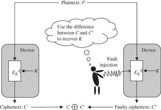
Figure 5.71 Overview of differential fault analysis
5.5.1.1 Fault Model
Fault model is an important concept for DFA. The fault model describes the consequence of a fault injection in the calculation of a cryptographic algorithm. For example, in a fault model for AES-128, it can be assumed that the attackers alter the value of 1 bit of the intermediate value at certain timing. If the position of 1-bit fault is unknown, the attackers need to assume ![]() possible faults.
possible faults.
With different fault models, the efficiency in the key recovery of DFA is largely varied. Under a specific fault model, the key recovery algorithm is highly related to the cryptanalysis introduced in Chapter 4. The reasonable fault models are the ones that can be achieved with a fault injection setup for real devices. In this regards, 1-byte fault is more reasonable compared to 1-bit fault in the previous example if the device performs on byte-oriented operations. Therefore, this section focuses on the fault model that the attackers alter the value of a byte of the intermediate value into a random faulty value. This fault model is called random byte-fault model. In this section, it is further assumed that the attackers can control the position of the altered byte. Chapter 6 will discuss the case that the position of the altered byte is unknown.
For the random byte-fault model in the fixed byte position, the possible difference between the fault-free intermediate value and the faulty intermediate value is restricted to a set of size ![]() . The only 1 active byte has
. The only 1 active byte has ![]() possible values in the difference, whereas the other inactive bytes have no difference.
possible values in the difference, whereas the other inactive bytes have no difference.
5.5.1.2 Key Recovery Concept of DFA on AES-128
The key recovery concept for DFA on AES-128 can be understood as follows. Under the random byte-fault model in the fixed byte position, the attackers know that there is 1 active byte at the position where the fault is injected. In addition, the attackers obtain the values of the fault-free and the faulty ciphertexts.
The attackers first prepare an expected propagation of the active bytes under the AES-128 specification. Then, the attackers guess subkey values in the last several rounds. For each key candidate, the attackers use the partial decryption of AES-128 with the fault-free and the faulty ciphertexts to calculate the origin of the active byte. In detail, using a key candidate and the fault-free ciphertext, the fault-free intermediate values can be calculated. Moreover, using the key candidate and the faulty ciphertext, the faulty intermediate values are calculated as well. Then the differences between the fault-free and the faulty intermediate values are calculated.
The calculated propagation of the active bytes using a key candidate is checked whether or not 1 active byte is located at an intended position specified by the fault model. If the calculated active byte position does not match the fault model, the corresponding key candidate can be discarded from the key space. After exhaustively checking all the possible key candidates, the key space can be narrowed down. In practice, this key recovery algorithm is optimized with divide-and-conquer algorithm to make the computational cost practical.
5.5.1.3 Propagation of Active Bytes in AES-128
The active bytes propagate in accordance with the specification of AES-128, which has been explained in Chapter 1. Here, the propagation of the active bytes by one AES round, which consists of ![]() ,
, ![]() ,
, ![]() , and
, and ![]() , is briefly reviewed.
, is briefly reviewed.
For the ![]() operation, the input and output states have the same number of active bytes at the same positions. Recall that AES S-box is bijective, which infers that two different S-box inputs never have the same output value. Thus, an active byte remains active after the
operation, the input and output states have the same number of active bytes at the same positions. Recall that AES S-box is bijective, which infers that two different S-box inputs never have the same output value. Thus, an active byte remains active after the ![]() operation.
operation.
For the ![]() operation, the input and output states have the same number of active bytes as only the positions of the active bytes are changed.
operation, the input and output states have the same number of active bytes as only the positions of the active bytes are changed.
For the ![]() operation, first recall that
operation, first recall that ![]() is a column-wise operation. The input and output columns related to the
is a column-wise operation. The input and output columns related to the ![]() operation have 8 bytes in total. An important feature is that these 8 bytes either have 0 active bytes or have 5 or more active bytes due to the property of MDS introduced in Chapter 4. Following this rule, one can see that if the input column of
operation have 8 bytes in total. An important feature is that these 8 bytes either have 0 active bytes or have 5 or more active bytes due to the property of MDS introduced in Chapter 4. Following this rule, one can see that if the input column of ![]() has 1 active byte, the output column must have 4 active bytes. Figure 5.72 shows some possible and impossible propagation patterns of the active bytes for the input and output columns of the
has 1 active byte, the output column must have 4 active bytes. Figure 5.72 shows some possible and impossible propagation patterns of the active bytes for the input and output columns of the ![]() operation.
operation.

Figure 5.72 Propagation patterns for each column of  calculation
For the ![]() operation, the active bytes keep their values of difference and positions as
operation, the active bytes keep their values of difference and positions as ![]() only performs XOR with a subkey.
only performs XOR with a subkey.
With the above-mentioned explanations, Figure 5.73 shows the propagation of the active bytes via 1 AES round starting with 1 active byte at ![]() . The 1 active byte at the AES round input remains active after the
. The 1 active byte at the AES round input remains active after the ![]() operation, changes its position after the
operation, changes its position after the ![]() operation, and propagates to 4 active bytes in the
operation, and propagates to 4 active bytes in the ![]() operation. After the
operation. After the ![]() operation, the AES round output has 4 active bytes in a column. The propagation of the active bytes follows Figure 5.73 regardless of the value of AES states and the secret key.
operation, the AES round output has 4 active bytes in a column. The propagation of the active bytes follows Figure 5.73 regardless of the value of AES states and the secret key.

Figure 5.73 Propagation of active bytes in one-round operation (encryption direction)
Let us see the propagation of 4 active bytes following the decryption direction of AES as shown in Figure 5.74. Suppose that 4 active bytes are located at one column in the output of the AES round, that is, ![]() . The active bytes at the input for the
. The active bytes at the input for the ![]() operation is the same as ones at
operation is the same as ones at ![]() . The active bytes at the input for the
. The active bytes at the input for the ![]() operation,
operation, ![]() , are uncertain owing to the property of MDS. According to the propagation rule of
, are uncertain owing to the property of MDS. According to the propagation rule of ![]() , the first column of
, the first column of ![]() could have 1, 2, 3, or 4 active bytes. Hence, the difference at
could have 1, 2, 3, or 4 active bytes. Hence, the difference at ![]() could have 1, 2, 3, or 4 active bytes as well. The number of active bytes and their positions at
could have 1, 2, 3, or 4 active bytes as well. The number of active bytes and their positions at ![]() requires the value of the key to be determined.
requires the value of the key to be determined.

Figure 5.74 Propagation of active bytes in one-round operation (decryption direction)
The DFA attack against first round of AES can be considered as follows. Suppose that the fault is injected to a fixed byte at the beginning of the AES round, ![]() , accordingly to the random byte-fault model. As shown in Figure 5.73, the number of active bytes and their positions are fixed at the output of the AES round. The fault-free value and the faulty value at
, accordingly to the random byte-fault model. As shown in Figure 5.73, the number of active bytes and their positions are fixed at the output of the AES round. The fault-free value and the faulty value at ![]() are denoted by C and
are denoted by C and ![]() , respectively. For a key candidate
, respectively. For a key candidate ![]() , the difference at
, the difference at ![]() can be calculated by
can be calculated by
If the result of ![]() does not have a difference at
does not have a difference at ![]() as shown in Figure 5.73, the current key candidate cannot be the correct key, and therefore it can be removed from the key space. Actually, the attackers only need to check the difference at
as shown in Figure 5.73, the current key candidate cannot be the correct key, and therefore it can be removed from the key space. Actually, the attackers only need to check the difference at ![]() as the propagation from
as the propagation from ![]() to
to ![]() is fixed in the decryption direction. Note that the MDS property of the
is fixed in the decryption direction. Note that the MDS property of the ![]() operation is the point for the key recovery of DFA on AES-128.
operation is the point for the key recovery of DFA on AES-128.
For the DFA attack on first round of AES explained above, only 4 bytes of ![]() are related to the active bytes at
are related to the active bytes at ![]() . Before the DFA attack, there are
. Before the DFA attack, there are ![]() possible key candidates. The size of the remaining key candidates after the DFA attack can be roughly estimated. In Figure 5.73, the number of the possible difference at
possible key candidates. The size of the remaining key candidates after the DFA attack can be roughly estimated. In Figure 5.73, the number of the possible difference at ![]() is
is ![]() . In contrast, the number of the possible values of the difference at
. In contrast, the number of the possible values of the difference at ![]() is
is ![]() . Thus, for a random mapping from the difference at
. Thus, for a random mapping from the difference at ![]() to the difference at
to the difference at ![]() , the probability of a match is estimated as
, the probability of a match is estimated as ![]() . Therefore, about
. Therefore, about ![]() , key candidates will remain after the DFA attack on one round of AES with one pair of fault-free and the faulty ciphertexts. The above-mentioned estimation matches the average of the experimental results.
, key candidates will remain after the DFA attack on one round of AES with one pair of fault-free and the faulty ciphertexts. The above-mentioned estimation matches the average of the experimental results.
5.5.1.4 DFA Attack on AES-128 with a Byte Fault at 
Let us consider the case where the fault is injected to a fixed byte at the beginning of the eighth AES round accordingly to the random byte-fault model. This fault model has been discussed in many literatures, such as Piret and Quisquater (2003), Tunstall et al. (2011) and Mukhopadhyay (2009). Following the encryption direction of the AES algorithm, the propagation of the active bytes is shown in Figure 5.75. The 1 active byte at ![]() will propagate to 4 active bytes at state
will propagate to 4 active bytes at state ![]() as a column. Then these 4 active bytes are distributed to 4 columns at
as a column. Then these 4 active bytes are distributed to 4 columns at ![]() . Each active byte at
. Each active byte at ![]() is propagated to 4 active bytes at the ciphertext. For example, the active bytes marked by bold lines correspond to the fourth column of the
is propagated to 4 active bytes at the ciphertext. For example, the active bytes marked by bold lines correspond to the fourth column of the ![]() operation of the ninth AES round, which are used as a group in the key recovery.
operation of the ninth AES round, which are used as a group in the key recovery.

Figure 5.75 Propagation of active bytes for AES-128
The key recovery algorithm for DFA on AES-128 is illustrated in Algorithm 5.10, which can be divided into two parts.
For the first part, that is, steps 1 to 10 in Algorithm 5.10, the key recovery considers only the last two rounds of AES, that is, ninth and tenth rounds. The key recovery is performed separately for each column of ![]() of the ninth round. With a key candidate of 4 bytes of
of the ninth round. With a key candidate of 4 bytes of ![]() that are related to 1 column of the
that are related to 1 column of the ![]() of the ninth round, the difference of this column at
of the ninth round, the difference of this column at ![]() can be calculated using C and
can be calculated using C and ![]() . The calculated difference is compared with the expected pattern of the active byte. For each column of
. The calculated difference is compared with the expected pattern of the active byte. For each column of ![]() of the ninth round, the size of the key space for the 4 bytes of
of the ninth round, the size of the key space for the 4 bytes of ![]() is expected to be
is expected to be ![]() as there are
as there are ![]() key candidates and the probability of a match is about
key candidates and the probability of a match is about ![]() . After the first part of the attack, the key space of
. After the first part of the attack, the key space of ![]() will be restricted to about
will be restricted to about ![]() or
or ![]() . The computational cost of the first part is about four times of exhaustive verifications of
. The computational cost of the first part is about four times of exhaustive verifications of ![]() key candidates, which can be computed by a standard personal computer.
key candidates, which can be computed by a standard personal computer.
The second part of the DFA attack on AES-128, that is, steps 11 to 18 in Algorithm 5.10, considers the last three rounds of AES. After the first part, the size of the remaining key space of ![]() is
is ![]() . For each key candidate of
. For each key candidate of ![]() , one can calculate the difference at
, one can calculate the difference at ![]() using C and
using C and ![]() . At the
. At the ![]() of the eighth round, the probability of a match is about
of the eighth round, the probability of a match is about ![]() . Thus, after the second part of the DFA attack, the size of the key space is narrowed down to around
. Thus, after the second part of the DFA attack, the size of the key space is narrowed down to around ![]() .
.
Finally, the attackers need some additional information to identify the key. One way to identify the key is to use a plaintext–ciphertext pair to verify all the remaining key candidates. The other way is to perform another fault injection and run Algorithm 5.10 again and prepare another set for the key candidates whose size is ![]() . The correct key can be identified with high probability by checking the intersection of those key candidate sets.
. The correct key can be identified with high probability by checking the intersection of those key candidate sets.
5.5.2 Fault Sensitivity Analysis 
This section discusses a relatively new type of fault analysis called fault sensitivity analysis (FSA). For FSA, the attackers use fault injections to obtain the information leakage called fault sensitivity (FS) from the device. FS describes how strong the intensity of a fault injection is required to successfully inject a fault in the target device. In other words, FS describes how much the current calculation is sensitive to the attempt of a fault injection. With the FS data, the key recovery algorithm used for side-channel analysis can be directly applied to achieve the key recovery in FSA.
A special feature of FSA compared to DFA is that the value of the faulty calculation result is not required to recover the key. This feature is useful to attack implementations with the countermeasures against the DFA attack, which ensures that the attackers cannot obtain the value of the faulty calculation result. This type of countermeasure is not effective against the FSA attack.
5.5.2.1 Fault Injection Intensity
To understand the FS, it is also required to understand the concept of fault injection intensity. In the default working environment of a device, no fault is expected for the calculation. When the attackers attempt to perform a fault injection, the working environment is changed. Fault injection intensity describes how much the environment is changed in the attempt of injecting a fault.
For a laser-based fault injection, the stronger the power level of the laser shot is, the higher the fault injection intensity is. For an under-power-based fault injection, the lower the voltage of the power supply is, the higher the fault injection intensity is. For an illegal clock-based fault injection, the shorter the period of the illegal clock cycle is, the higher the fault injection intensity is. In general, the larger the potential of a faulty calculation is, the higher the fault injection intensity is.
Figure 5.76 shows an example of the fault injection intensity for the illegal clock signal. There are four clock signals listed in Figure 5.76, from clock signals 1 to 4, the clock period of the illegal clock cycle decreases gradually. Thus, the fault injection intensity gradually increases.

Figure 5.76 Fault injection intensity for illegal clock signal
5.5.2.2 Critical Fault Injection Intensity as Fault Sensitivity
In practice, FS is measured as the critical fault injection intensity. FSA assumes that the same calculation, for example, the encryption of the same plaintext, is repeated under the fault injections with controlled fault injection intensities. It is possible for the attackers to understand the threshold of the fault injection intensity between the device's normal and abnormal behaviors, which is the critical fault injection intensity or FS. When the fault injection intensity is lower than the FS, the device performs the correct calculation and outputs the fault-free calculation result. When the fault injection intensity is higher than the FS, the device performs a faulty calculation and outputs a faulty calculation result.
In Figure 5.77, the measurement of FS using illegal clock signals is illustrated. For plaintext ![]() , the encryption is repeated four times with clock signals 1 to 4. The encryption results using clock signals 1 to 3 are the same with each other, and the encryption result using clock signal 4 is a different value that is a faulty value. One can see that for plaintext
, the encryption is repeated four times with clock signals 1 to 4. The encryption results using clock signals 1 to 3 are the same with each other, and the encryption result using clock signal 4 is a different value that is a faulty value. One can see that for plaintext ![]() , the clock signal 4 is the threshold to trigger the faulty ciphertext output. For plaintext
, the clock signal 4 is the threshold to trigger the faulty ciphertext output. For plaintext ![]() , the same process is performed and the clock signal 3 is the threshold to trigger the faulty ciphertext output.
, the same process is performed and the clock signal 3 is the threshold to trigger the faulty ciphertext output.

Figure 5.77 Fault sensitivity measured as critical fault injection intensity
As shown in Figure 5.77, by varying the fault injection intensity and observing the calculation results, the FS can be measured. In practice, for different data, the measured fault sensitivities are expected to be different. In the example shown in Figure 5.77, the calculation using ![]() is more sensitive to the fault injections compared to that of
is more sensitive to the fault injections compared to that of ![]() . The difference of FS when processing different data is the point of the key recovery in FSA.
. The difference of FS when processing different data is the point of the key recovery in FSA.
When illegal clock signal is used in the FSA attack, the setup-time violations occur in the device. Thus, the measured FS data is related to the path delay of a calculation in the clock cycle. For the setup-time violation, whether a fault occurs depends on the relations between the path delay ![]() and the clock period
and the clock period ![]() . The attackers control
. The attackers control ![]() and observe the calculation results to measure the FS that is related to
and observe the calculation results to measure the FS that is related to ![]() . As
. As ![]() is related to the processed data, the measured FS is related to the processed data as well.
is related to the processed data, the measured FS is related to the processed data as well.
5.5.2.3 Data Dependency of Signal Delays
A simple example is given to show that the path delays of signals depend on the value of the processed data. Consider a two-input AND gate with input signals A and B and the output signal C = ![]() . Assume that the signal A always arrives earlier than the signal B to the AND gate, that is,
. Assume that the signal A always arrives earlier than the signal B to the AND gate, that is, ![]() .
.
Assume that the initial values of A and B are both 1 and they are transmitted into the next values in a certain clock cycle. The path delay of C, ![]() , is discussed for four possible cases of the next values of A and B as shown in Figure 5.78.
, is discussed for four possible cases of the next values of A and B as shown in Figure 5.78.
- When the next values of A and B are
 and
and  , the next value of C is determined when signal A arrives at the AND gate as a zero input already decides the output of the AND gate. Thus,
  is determined only with
  , that is,
  .
. - When the next values of A and B are
 and
and  , similarly
  is determined only with
  , that is,
  .
. - When the next values of A and B are
 and
and  , the next value of C is determined when signal B arrives at the AND gate. Thus,
  is determined with
  , that is,
  .
. - When the next values of A and B are
 and
and  , the next value of C is not changed from the initial value. Thus,
  .
.
From the above-mentioned discussion, it is confirmed that the path delay of the AND gate largely depends on the values of the input signals. Note that the delay of the AND gate itself is ignored in the above-mentioned discussion for simplicity.

Figure 5.78 Example of data dependency of path delays
Table 5.2 Signal transitions and path delay for AND gate
| A | B | C | |
5.5.2.4 Collection of Fault Sensitivity Data
The first task for the attackers to perform the FSA attack is to collect the FS data. The method is written in Algorithm 5.11, where F denotes the fault injection intensity. For each plaintext as the input, the encryption requires to be performed several times. For the first encryption as shown in step 4 in Algorithm 5.11, no fault injection is performed, that is, ![]() . Then in steps 6 and 7, the encryption is repeated several times until the encryption has a fault successfully injected. For each repetition of the encryption, the fault injection intensity F is increased by a certain amount. For example, one can shorten the period of the illegal clock cycle by 5%. The fault injection intensity that corresponds to the successful fault injection is stored as the FS as shown in step 9 in Algorithm 5.11.
. Then in steps 6 and 7, the encryption is repeated several times until the encryption has a fault successfully injected. For each repetition of the encryption, the fault injection intensity F is increased by a certain amount. For example, one can shorten the period of the illegal clock cycle by 5%. The fault injection intensity that corresponds to the successful fault injection is stored as the FS as shown in step 9 in Algorithm 5.11.
When AES-128 is the target of FSA, the attackers can perform the fault injection at the last round of AES so that FS of the last round AES calculation can be measured. Note that the measured FS data is not in the form of a trace. The FS data can be measured for each S-box in the last AES round independently by observing the correctness of each byte of ciphertext independently. Therefore, each ![]() ,
, ![]() , in Algorithm 5.11 can be extended to a set of 16 FS data corresponding to 16 S-boxes, that is,
, in Algorithm 5.11 can be extended to a set of 16 FS data corresponding to 16 S-boxes, that is, ![]() .
.
5.5.2.5 FSA Key Recovery Algorithm Using LMs
After the collection of FS data, the attackers use the key recovery algorithm to identify the secret key. Similar to the side-channel information such as the power consumption, the FS data also depends on the processed intermediate value during the cryptographic algorithm. Thus, the key recovery techniques used in side-channel analysis can be applied to the FSA attack. This section explains the FSA key recovery algorithm based on the LMs. One can review Section 5.8 to recall the general DPA key recovery algorithm.
First of all, the key recovery is performed with divide-and-conquer algorithm. For AES, the key is usually recovered byte by byte. The attackers first guess the value of the target key byte as G. Then the key guess G is used with the public data such as ciphertexts to calculate the target intermediate values using the ![]() . The calculated target intermediate values are used with an
. The calculated target intermediate values are used with an ![]() to obtain the temporary results, T. The calculated T is compared with the measured FS data using an EF, and the evaluation result is obtained. For each possible key guess, the mentioned calculation for obtaining the evaluation result is performed. The attackers know the expected result of the evaluation for the correct key guess. Thus, the attackers compare the evaluation results for all key candidates and pick up the one that is the most likely to be the correct key as the attack result.
to obtain the temporary results, T. The calculated T is compared with the measured FS data using an EF, and the evaluation result is obtained. For each possible key guess, the mentioned calculation for obtaining the evaluation result is performed. The attackers know the expected result of the evaluation for the correct key guess. Thus, the attackers compare the evaluation results for all key candidates and pick up the one that is the most likely to be the correct key as the attack result.
The key recovery algorithm using FS data targeting the first byte of ![]() of AES-128 is shown in Algorithm 5.12. For each key candidate of G, the rough estimation of the FS data is performed by
of AES-128 is shown in Algorithm 5.12. For each key candidate of G, the rough estimation of the FS data is performed by ![]() , in which
, in which ![]() is the calculation of the target intermediate value with the SF. As for the LM used in step 3in Algorithm 5.12, the LMs such as the HW and HD models can be used. The effectiveness of the used LM largely depends on the implementation method.
is the calculation of the target intermediate value with the SF. As for the LM used in step 3in Algorithm 5.12, the LMs such as the HW and HD models can be used. The effectiveness of the used LM largely depends on the implementation method.
- It is found that for the FSA attack against AES-pprm1, the HW model is an effective LM. There is an array of AND gates at the beginning of the S-box of AES-pprm1. For each AND gate, the output can be determined if any of the inputs is determined to be zero. Each zero input to an AND gate has a potential to make the output gets determined earlier. Therefore, in general, the output of the AND gate array is like to get determined earlier when the input has more zero bits.
- It is also found that clockwise collision model is effective for the FSA attack on AES-comp as the clockwise collision leads to not only a low-power consumption but also a short path delay for the AES-comp S-box.
In Algorithm 5.12, the correlation between the rough estimation of the FS data and the measured FS data is used as the EF. Only when G is the real one, the calculated intermediate values are correct; thus, the estimated FS data can be expected to be correlated with the measured FS data. Thus, the key guess that corresponds to the highest correlation is expected to be the correct key as shown in step 9 in Algorithm 5.12. Note that Algorithm 5.12 is similar to the key recovery algorithms for previously introduced side-channel analysis.
5.5.2.6 FSA Key Recovery Algorithm Using Collision Model
When there is no appropriate LM for the FSA attack, it is natural to consider using the collision model in the key recovery. In the collision model, the attackers do not care about the relations between the intermediate value and the FS data. The attackers take advantages of the fact that when two S-boxes of the same implementation have the same input value, the FS of the S-box calculations is similar to each other. One can review Section 5.3.8 to recall the power analysis using the collision model.
The key recovery algorithm using collision model for AES-128 is written in Algorithm 5.13 for the FSA attack, which was proposed in Moradi et al. (2011). The target is set to the difference between the first two key bytes of the last round key, that is, ![]() . Two group separations for
. Two group separations for ![]() and
and ![]() are performed according to the values of
are performed according to the values of ![]() and
and ![]() , respectively. For the 256 groups for group separation 1, the means of the FS data are calculated as
, respectively. For the 256 groups for group separation 1, the means of the FS data are calculated as ![]() ,
, ![]() . For the 256 groups for group separation 2, the means of the FS data are calculated as
. For the 256 groups for group separation 2, the means of the FS data are calculated as ![]() ,
, ![]() .
.
With a guess of the key byte difference ![]() , the correlation between
, the correlation between ![]() and
and ![]() for
for ![]() is calculated. When
is calculated. When ![]() is the same with the real one, each pair of
is the same with the real one, each pair of ![]() and
and ![]() for any i is a pair of FS data for two S-boxes with the same input value. Thus, a high correlation is expected for the correct
for any i is a pair of FS data for two S-boxes with the same input value. Thus, a high correlation is expected for the correct ![]() . To understand this, recall that the related two S-box inputs of the last AES round can be calculated as
. To understand this, recall that the related two S-box inputs of the last AES round can be calculated as ![]() and
and ![]() . These two S-box inputs are the same if
. These two S-box inputs are the same if
or
In addition, recall that the ciphertexts for ![]() satisfy
satisfy ![]() , and the ciphertexts for
, and the ciphertexts for ![]() satisfy
satisfy ![]() . When
. When ![]() , for
, for ![]() and
and ![]() , it is satisfied that
, it is satisfied that
Thus, for ![]() and
and ![]() , the S-box inputs are the same when
, the S-box inputs are the same when ![]() is the same with the real one. At step 14 in Algorithm 5.13, the
is the same with the real one. At step 14 in Algorithm 5.13, the ![]() corresponding to the highest correlation is set to the attack result.
corresponding to the highest correlation is set to the attack result.
The successful key recovery of the FSA attack using collision model has been applied to many AES implementations. On the one hand, with the FSA attack using collision model, the attackers' required knowledge for a successful key recovery is largely reduced. On the other hand, as shown in both Algorithms 5.12 and 5.13, the value of the faulty ciphertext ![]() is not used in the key recovery of FSA. Therefore, some DFA countermeasures are also valid targets under the attack concept of the FSA attack.
is not used in the key recovery of FSA. Therefore, some DFA countermeasures are also valid targets under the attack concept of the FSA attack.
Acknowledgment
The authors greatly appreciate Prof. Tsutomu Matsumoto at Yokohama National University, Japan, for kind permission to use the power consumption data measured in his research group, which can be found at (Research Center for Information and Physical Security, Yokohama National University). It highly enhanced the accomplishment level of this chapter.
Bibliography
- Ali S and Mukhopadhyay D 2011 A Differential Fault Analysis on AES Key Schedule Using Single Fault In FDTC (ed. Breveglieri L, Guilley S, Koren I, Naccache D and Takahashi J), pp. 35–42. IEEE.
- Brier E, Clavier C and Olivier F 2004 Correlation power analysis with a leakage model. CHES 2004, vol. 3156 of Lecture Notes in Computer Science, pp. 16–29. Springer-Verlag.
- Kocher PC, Jaffe J and Jun B 1999 Differential power analysis CRYPTO 1999, vol. 1666 of Lecture Notes in Computer Science, pp. 388–397. Springer-Verlag.
- Moradi A, Mischke O and Eisenbarth T 2010 Correlation-enhanced power analysis collision attack In CHES (ed. Mangard S and Standaert FX), vol. 6225 of Lecture Notes in Computer Science, pp. 125–139. Springer-Verlag.
- Moradi A, Mischke O, Paar C, Li Y, Ohta K and Sakiyama K 2011 On the power of fault sensitivity analysis and collision side-channel attacks in a combined setting In CHES (ed. Preneel B and Takagi T), vol. 6917 of Lecture Notes in Computer Science, pp. 292–311. Springer-Verlag.
- Morioka S and Satoh A 2002 An optimized S-box circuit architecture for low power AES design In CHES (ed. Kaliski BS Jr., Koç ÇK and Paar C), vol. 2523 of Lecture Notes in Computer Science, pp. 172–186. Springer-Verlag.
- Mukhopadhyay D 2009 An improved fault based attack of the advanced encryption standard In AFRICACRYPT (ed. Preneel B), vol. 5580 of Lecture Notes in Computer Science, pp. 421–434. Springer-Verlag.
- Piret G and Quisquater JJ 2003 A differential fault attack technique against SPN structures, with application to the AES and KHAZAD CHES 2003, vol. 2779 of Lecture Notes in Computer Science, pp. 77–88. Springer-Verlag.
- Research Center for Information and Physical Security, Yokohama National University n.d. Power Consumption Data Measured Using LSI on SASEBO-R http://ipsr.ynu.ac.jp/wxf/index.html.
- Satoh A, Morioka S, Takano K and Munetoh S 2001 A compact Rijndael hardware architecture with S-box optimization In ASIACRYPT (ed. Boyd C), vol. 2248 of Lecture Notes in Computer Science, pp. 239–254. Springer-Verlag.
- Tunstall M, Mukhopadhyay D and Ali S 2011 Differential fault analysis of the advanced encryption standard using a single fault In Information Security Theory and Practice. Security and Privacy of Mobile Devices in Wireless Communication (ed. Ardagna C and Zhou J), vol. 6633 of Lecture Notes in Computer Science, pp. 224–233. Springer-Verlag Berlin and Heidelberg.