2

Data Preprocessing

You often hear in the data science industry that a data scientist typically spends close to 80% of their time on getting the data, processing it, cleaning it, and so on. And only then the remaining 20% of the time is actually spent on modeling, which is often considered to be the most interesting part. In the previous chapter, we have already learned how to download data from various sources. We still need to go through a few steps before we can draw actual insights from the data.

In this chapter, we will cover data preprocessing, that is, general wrangling/manipulation applied to the data before using it. The goal is not only to enhance the model’s performance but also to ensure the validity of any analysis based on that data. In this chapter, we will focus on the financial time series, while in the subsequent chapters, we will also show how to work with other kinds of data.

In this chapter, we cover the following recipes:

• Converting prices to returns
• Adjusting the returns for inflation
• Changing the frequency of time series data
• Different ways of imputing missing data
• Changing currencies
• Different ways of aggregating trade data

Converting prices to returns

Many of the models and approaches used for time series modeling require the time series to be stationary. We will cover that topic in depth in Chapter 6, Time Series Analysis and Forecasting, however, we can get a quick glimpse of it now.

Stationarity assumes that the statistics (mathematical moments) of a process, such as the series’ mean and variance, do not change over time. Using that assumption, we can build models that aim to forecast the future values of the process.

However, asset prices are usually non-stationary. Their statistics not only change over time, but we can also observe some trends (general patterns over time) or seasonality (patterns repeating over fixed time intervals). By transforming the prices into returns, we attempt to make the time series stationary.

Another benefit of using returns, as opposed to prices, is normalization. It means that we can easily compare various return series, which would not be that simple with raw stock prices, as one stock might start selling at $10, while another at $1,000.

There are two types of returns:

• Simple returns: They aggregate over assets—the simple return of a portfolio is the weighted sum of the returns of the individual assets in the portfolio. Simple returns are defined as:

  R_t = (P_t - P_t-1)/P_t-1 = P_t/P_t-1 -1

• Log returns: They aggregate over time. It is easier to understand with the help of an example—the log return for a given month is the sum of the log returns of the days within that month. Log returns are defined as:

  r_t = log(P_t/P_t-1) = log(P_t) - log(P_t-1)

P_t is the price of an asset in time t. In the preceding case, we do not consider dividends, which obviously impact the returns and require a small modification of the formulas.

In general, log returns are often preferred over simple returns. Probably the most important reason for that is the fact that if we assume that the stock prices are log-normally distributed (which might or might not be the case for the particular time series), then the log returns would be normally distributed. And the normal distribution would work well with quite a lot of classic statistical approaches to time series modeling. Also, the difference between simple and log returns for daily/intraday data will be very small, in accordance with the general rule that log returns are smaller in value than simple returns.

In this recipe, we show how to calculate both types of returns using Apple’s stock prices.

How to do it…

Execute the following steps to download Apple’s stock prices and calculate simple/log returns:

1. Import the libraries:

   import pandas as pd
   import numpy as np
   import yfinance as yf
   
2. Download the data and keep the adjusted close prices only:

   df = yf.download("AAPL",
                    start="2010-01-01",
                    end="2020-12-31",
                    progress=False)
   df = df.loc[:, ["Adj Close"]]
   
3. Calculate the simple and log returns using the adjusted close prices:

   df["simple_rtn"] = df["Adj Close"].pct_change()
   df["log_rtn"] = np.log(df["Adj Close"]/df["Adj Close"].shift(1))
   
4. Inspect the output:

   df.head()
   

   The resulting DataFrame looks as follows:

Figure 2.1: Snippet of the DataFrame containing Apple’s adjusted close prices and simple/log returns

The first row will always contain a NaN (not a number) value, as there is no previous price to use for calculating the returns.

How it works…

In Step 2, we downloaded price data from Yahoo Finance and only kept the adjusted close price for the calculation of the returns.

To calculate the simple returns, we used the pct_change method of pandas Series/DataFrame. It calculates the percentage change between the current and prior element (we can specify the number of lags, but for this specific case the default value of 1 suffices). Please bear in mind that the prior element is defined as the one in the row above the given row. In the case of working with time series data, we need to make sure that the data is sorted by the time index.

To calculate the log returns, we followed the formula given in the introduction to this recipe. When dividing each element of the series by its lagged value, we used the shift method with a value of 1 to access the prior element. In the end, we took the natural logarithm of the divided values by using the np.log function.

Adjusting the returns for inflation

When doing different kinds of analyses, especially long-term ones, we might want to consider inflation. Inflation is the general rise of the price level of an economy over time. Or to phrase it differently, the reduction of the purchasing power of money. That is why we might want to decouple the inflation from the increase of the stock prices caused by, for example, the companies’ growth or development.

We can naturally adjust the prices of stocks directly, but in this recipe, we will focus on adjusting the returns and calculating the real returns. We can do so using the following formula:

where R^r_t is the real return, R_t is the time t simple return, and stands for the inflation rate.

For this example, we use Apple’s stock prices from the years 2010 to 2020 (downloaded as in the previous recipe).

How to do it…

Execute the following steps to adjust the returns for inflation:

1. Import libraries and authenticate:

   import pandas as pd
   import nasdaqdatalink
   nasdaqdatalink.ApiConfig.api_key = "YOUR_KEY_HERE"
   
2. Resample daily prices to monthly:

   df = df.resample("M").last()
   
3. Download inflation data from Nasdaq Data Link:

   df_cpi = (
       nasdaqdatalink.get(dataset="RATEINF/CPI_USA", 
                          start_date="2009-12-01", 
                          end_date="2020-12-31")
       .rename(columns={"Value": "cpi"})
   )
   df_cpi
   

   Running the code generates the following table:

   

   Figure 2.2: Snippet of the DataFrame containing the values of the Consumer Price Index (CPI)

4. Join inflation data to prices:

   df = df.join(df_cpi, how="left")
   
5. Calculate simple returns and inflation rate:

   df["simple_rtn"] = df["Adj Close"].pct_change()
   df["inflation_rate"] = df["cpi"].pct_change()
   
6. Adjust the returns for inflation and calculate the real returns:

   df["real_rtn"] = (
       (df["simple_rtn"] + 1) / (df["inflation_rate"] + 1) - 1
   )
   df.head()
   

   Running the code generates the following table:

Figure 2.3: Snippet of the DataFrame containing the calculated inflation-adjusted returns

How it works…

First, we imported the libraries and authenticated with Nasdaq Data Link, which we used for downloading the inflation-related data. Then, we had to resample Apple’s stock prices to a monthly frequency, as the inflation data is provided monthly. To do so, we chained the resample method with the last method. This way, we took the last price of the given month.

In Step 3, we downloaded the monthly Consumer Price Index (CPI) values from Nasdaq Data Link. It is a metric that examines the weighted average of prices of a basket of consumer goods and services, such as food, transportation, and so on.

Then, we used a left join to merge the two datasets (prices and CPI). A left join is a type of operation used for merging tables that returns all rows from the left table and the matched rows from the right table while leaving the unmatched rows empty.

By default, the join method uses the indices of the tables to carry out the actual joining. We can use the on argument to specify which column/columns to use otherwise.

Having all the data in one DataFrame, we used the pct_change method to calculate the simple returns and the inflation rate. Lastly, we used the formula presented in the introduction to calculate the real returns.

There’s more…

We have already explored how to download the inflation data from Nasdaq Data Link. Alternatively, we can use a handy library called cpi.

1. Import the library:

   import cpi
   

   At this point, we might encounter the following warning:

   StaleDataWarning: CPI data is out of date
   

   If that is the case, we just need to run the following line of code to update the data:

   cpi.update()
   

2. Obtain the default CPI series:

   cpi_series = cpi.series.get()
   

   Here we download the default CPI index (CUUR0000SA0: All items in U.S. city average, all urban consumers, not seasonally adjusted), which will work for most of the cases. Alternatively, we can provide the items and area arguments to download a more tailor-made series. We can also use the get_by_id function to download a particular CPI series.

3. Convert the object into a pandas DataFrame:

   df_cpi_2 = cpi_series.to_dataframe()
   
4. Filter the DataFrame and view the top 12 observations:

   df_cpi_2.query("period_type == 'monthly' and year >= 2010") 
           .loc[:, ["date", "value"]] 
           .set_index("date") 
           .head(12)
   

   Running the code generates the following output:

Figure 2.4: The first 12 values of the DataFrame containing the downloaded values of the CPI

In this step, we used some filtering to compare the data to the data downloaded before from Nasdaq Data Link. We used the query method to only keep the monthly data from the year 2010 onward. We displayed only two selected columns and the first 12 observations, for comparison’s sake.

We will also be using the cpi library in later chapters to directly inflate the prices using the inflate function.

See also

• https://github.com/palewire/cpi—the GitHub repo of the cpi library

Changing the frequency of time series data

When working with time series, and especially financial ones, we often need to change the frequency (periodicity) of the data. For example, we receive daily OHLC prices, but our algorithm works with weekly data. Or we have daily alternative data, and we want to match it with our live feed of intraday data.

The general rule of thumb for changing frequency can be broken down into the following:

• Multiply/divide the log returns by the number of time periods.
• Multiply/divide the volatility by the square root of the number of time periods.

In this recipe, we present an example of how to calculate the monthly realized volatilities for Apple using daily returns and then annualize the values. We can often encounter annualized volatility when looking at the risk-adjusted performance of an investment.

The formula for realized volatility is as follows:

Realized volatility is frequently used for calculating the daily volatility using intraday returns.

The steps we need to take are as follows:

• Download the data and calculate the log returns
• Calculate the realized volatility over the months
• Annualize the values by multiplying by , as we are converting from monthly values

Getting ready

We assume you have followed the instructions from the previous recipes and have a DataFrame called df with a single log_rtn column and timestamps as the index.

How to do it…

Execute the following steps to calculate and annualize the monthly realized volatility:

1. Import the libraries:

   import pandas as pd
   import numpy as np
   
2. Define the function for calculating the realized volatility:

   def realized_volatility(x):
       return np.sqrt(np.sum(x**2))
   
3. Calculate the monthly realized volatility:

   df_rv = (
       df.groupby(pd.Grouper(freq="M"))
       .apply(realized_volatility)
       .rename(columns={"log_rtn": "rv"})
   )
   
4. Annualize the values:

   df_rv.rv = df_rv["rv"] * np.sqrt(12)
   
5. Plot the results:

   fig, ax = plt.subplots(2, 1, sharex=True)
   ax[0].plot(df)
   ax[0].set_title("Apple's log returns (2000-2012)")
   ax[1].plot(df_rv)
   ax[1].set_title("Annualized realized volatility")
   plt.show()
   

   Executing the snippet results in the following plots:

Figure 2.5: Apple’s log return series and the corresponding realized volatility (annualized)

We can see that the spikes in the realized volatility coincide with some extreme returns (which might be outliers).

How it works…

Normally, we could use the resample method of a pandas DataFrame. Supposing we wanted to calculate the average monthly return, we could use df["log_rtn"].resample("M").mean().

With the resample method, we can use any built-in aggregate function of pandas, such as mean, sum, min, and max. However, our case at hand is a bit more complex so we first defined a helper function called realized_volatility. Because we wanted to use a custom function for aggregation, we replicated the behavior of resample by using a combination of groupby, Grouper, and apply.

We presented the most basic visualization of the results (please refer to Chapter 3, Visualizing Financial Time Series, for information about visualizing time series).

Different ways of imputing missing data

While working with any time series, it can happen that some data is missing, due to many possible reasons (someone forgot to input the data, a random issue with the database, and so on). One of the available solutions would be to discard observations with missing values. However, imagine a scenario in which we are analyzing multiple time series at once, and only one of the series is missing a value due to some random mistake. Do we still want to remove all the other potentially valuable pieces of information because of this single missing value? Probably not. And there are many other potential scenarios in which we would rather treat the missing values somehow, rather than discarding those observations.

Two of the simplest approaches to imputing missing time series data are:

• Backward filling—fill the missing value with the next known value
• Forward filling—fill the missing value with the previous known value

In this recipe, we show how to use those techniques to easily deal with missing values in the example of the CPI time series.

How to do it…

Execute the following steps to try out different ways of imputing missing data:

1. Import the libraries:

   import pandas as pd
   import numpy as np
   import nasdaqdatalink
   
2. Download the inflation data from Nasdaq Data Link:

   nasdaqdatalink.ApiConfig.api_key = "YOUR_KEY_HERE"
    df = (
       nasdaqdatalink.get(dataset="RATEINF/CPI_USA", 
                          start_date="2015-01-01", 
                          end_date="2020-12-31")
       .rename(columns={"Value": "cpi"})
   )
   
3. Introduce five missing values at random:

   np.random.seed(42)
   rand_indices = np.random.choice(df.index, 5, replace=False)
   df["cpi_missing"] = df.loc[:, "cpi"]
   df.loc[rand_indices, "cpi_missing"] = np.nan
   df.head()
   

   In the following table, we can see we have successfully introduced missing values into the data:

Figure 2.6: Preview of the DataFrame with downloaded CPI data and the added missing values

4. Fill in the missing values using different methods:

   for method in ["bfill", "ffill"]:
       df[f"method_{method}"] = (
           df[["cpi_missing"]].fillna(method=method)
       )
   
5. Inspect the results by displaying the rows in which we created the missing values:

   df.loc[rand_indices].sort_index()
   

   Running the code results in the following output:

   

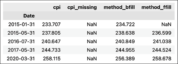
   Figure 2.7: Preview of the DataFrame after imputing the missing values

   We can see that backward filling worked for all the missing values we created. However, forward filling failed to impute one value. That is because this is the first data point in the series, so there is no available value to fill forward.

6. Plot the results for the years 2015 to 2016:

   df.loc[:"2017-01-01"] 
     .drop(columns=["cpi_missing"]) 
     .plot(title="Different ways of filling missing values");
   

   Running the snippet generates the following plot:

Figure 2.8: The comparison of backward and forward filling on the CPI time series

In Figure 2.8, we can clearly see how both forward and backward filling work in practice.

How it works…

After importing the libraries, we downloaded the 6 years of monthly CPI data from Nasdaq Data Link. Then, we selected 5 random indices from the DataFrame to artificially create missing values. To do so, we replaced those values with NaNs.

In Step 4, we applied two different imputation methods to our time series. We used the fillna method of a pandas DataFrame and specified the method argument as bfill (backward filling) or ffill (forward filling). We saved the imputed series as new columns, in order to clearly compare the results. Please remember that the fillna method replaces the missing values and keeps the other values intact.

Instead of providing a method of filling the missing data, we could have specified a value of our choice, for example, 0 or 999. However, using an arbitrary number might not make much sense in the case of time series data, so that is not advised.

In Step 5, we inspected the imputed values. For brevity, we have only displayed the indices we have randomly selected. We used the sort_index method to sort them by the date. This way, we can clearly see that the first value was not filled using the forward filling, as it is the very first observation in the time series.

Lastly, we plotted all the time series from the years 2015 to 2016. In the plot, we can clearly see how backward/forward filling imputes the missing values.

There’s more…

In this recipe, we have explored some simple methods of imputing missing data. Another possibility is to use interpolation, to which there are many different approaches. As such, in this example, we will use the linear one. Please refer to the pandas documentation (the link is available in the See also subsection) for more information about the available methods of interpolation.

1. Use linear interpolation to fill the missing values:

   df["method_interpolate"] = df[["cpi_missing"]].interpolate()
   
2. Inspect the results:

   df.loc[rand_indices].sort_index()
   

   Running the snippet generates the following output:

   

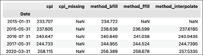
   Figure 2.9: Preview of the DataFrame after imputing the missing values with linear interpolation

   Unfortunately, linear interpolation also cannot deal with the missing value located at the very beginning of the time series.

3. Plot the results:

   df.loc[:"2017-01-01"] 
     .drop(columns=["cpi_missing"]) 
     .plot(title="Different ways of filling missing values");
   

   Running the snippet generates the following plot:

Figure 2.10: The comparison of backward and forward filling on the CPI time series, including interpolation

In Figure 2.10, we can see how linear interpolation connects the known observations with a straight line to impute the missing value.

In this recipe, we explored imputing missing data for time series data. However, these are not all of the possible approaches. We could have, for example, used the moving average of the last few observations to impute any missing values. There are certainly a lot of possible methodologies to choose from. In Chapter 13, Applied Machine Learning: Identifying Credit Default, we will show how to approach the issue of missing values for other kinds of datasets.

See also

• https://pandas.pydata.org/docs/reference/api/pandas.DataFrame.interpolate.html—here you can see all the available methods of interpolating available in pandas.

Converting currencies

Another quite common preprocessing step you might encounter while working on financial tasks is converting currencies. Imagine you have a portfolio of multiple assets, priced in different currencies and you would like to arrive at a total portfolio’s worth. The simplest example might be American and European stocks.

In this recipe, we show how to easily convert stock prices from USD to EUR. However, the very same steps can be used to convert any pair of currencies.

How to do it…

Execute the following steps to convert stock prices from USD to EUR:

1. Import the libraries:

   import pandas as pd
   import yfinance as yf
   from forex_python.converter import CurrencyRates
   
2. Download Apple’s OHLC prices from January 2020:

   df = yf.download("AAPL",
                    start="2020-01-01",
                    end="2020-01-31",
                    progress=False)
   df = df.drop(columns=["Adj Close", "Volume"])
   
3. Instantiate the CurrencyRates object:

   c = CurrencyRates()
   
4. Download the USD/EUR rate for each required date:

   df["usd_eur"] = [c.get_rate("USD", "EUR", date) for date in df.index]
   
5. Convert the prices in USD to EUR:

   for column in df.columns[:-1]:
       df[f"{column}_EUR"] = df[column] * df["usd_eur"]
   df.head()
   

   Running the snippet generates the following preview:

Figure 2.11: Preview of the DataFrame containing the original prices in USD and the ones converted to EUR

We can see that we have successfully converted all four columns with prices into EUR.

How it works…

In Step 1, we have imported the required libraries. Then, we downloaded Apple’s OHLC prices from January 2020 using the already covered yfinance library.

In Step 3, we instantiated the CurrencyRates object from the forex-python library. Under the hood, the library is using the Forex API (https://theforexapi.com), which is a free API for accessing current and historical foreign exchange rates published by the European Central Bank.

In Step 4, we used the get_rate method to download the USD/EUR exchange rates for all the dates available in the DataFrame with stock prices. To do so efficiently, we used list comprehension and stored the outputs in a new column. One potential drawback of the library and the present implementation is that we need to download each and every exchange rate individually, which might not be scalable for large DataFrames.

In the last step, we iterated over the columns of the initial DataFrame (all except the exchange rate) and multiplied the USD price by the exchange rate. We stored the outcomes in new columns, with _EUR subscript.

There’s more…

Using the forex_python library, we can easily download the exchange rates for many currencies at once. To do so, we can use the get_rates method. In the following snippet, we download the current exchange rates of USD to the 31 available currencies. We can naturally specify the date of interest, just as we have done before.

1. Get the current USD exchange rates to 31 available currencies:

   usd_rates = c.get_rates("USD")
   usd_rates
   

   The first five entries look as follows:

   {'EUR': 0.8441668073611345,
    'JPY': 110.00337666722943,
    'BGN': 1.651021441836907,
    'CZK': 21.426641904440316,
    'DKK': 6.277224379537396,
   }
   

   In this recipe, we have mostly focused on the forex_python library, as it is quite handy and flexible. However, we might download historical exchange rates from many different sources and arrive at the same results (accounting for some margin of error depending on the data provider). Quite a few of the data providers described in Chapter 1, Acquiring Financial Data, provide historical exchange rates. Below, we show how to get those rates using Yahoo Finance.

2. Download the USD/EUR exchange rate from Yahoo Finance:

   df = yf.download("USDEUR=X",
                    start="2000-01-01",
                    end="2010-12-31",
                    progress=False)
   df.head()
   

   Running the snippet results in the following output:

Figure 2.12: Preview of the DataFrame with the downloaded exchange rates

In Figure 2.12, we can see one of the limitations of this data source—the data for this currency pair is only available since December 2003. Also, Yahoo Finance is providing the OHLC variant of the exchange rates. To arrive at a single number used for conversion, you can pick any of the four values (depending on the use case) or calculate the mid-value (the middle between low and high values).

See also

• https://github.com/MicroPyramid/forex-python—the GitHub repo of the forex-python library

Different ways of aggregating trade data

Before diving into building a machine learning model or designing a trading strategy, we not only need reliable data, but we also need to aggregate it into a format that is convenient for further analysis and appropriate for the models we choose. The term bars refers to a data representation that contains basic information about the price movements of any financial asset. We have already seen one form of bars in Chapter 1, Acquiring Financial Data, in which we explored how to download financial data from a variety of sources.

There, we downloaded OHLCV data sampled by some time period, be it a month, day, or intraday frequencies. This is the most common way of aggregating financial time series data and is known as the time bars.

There are some drawbacks of sampling financial time series by time:

• Time bars disguise the actual rate of activity in the market—they tend to oversample low activity periods (for example, noon) and undersample high activity periods (for example, close to market open and close).
• Nowadays, markets are more and more controlled by trading algorithms and bots, so they no longer follow human daylight cycles.
• Time-based bars offer poorer statistical properties (for example, serial correlation, heteroskedasticity, and non-normality of returns).
• Given that this is the most popular kind of aggregation and the easiest one to access, it can also be prone to manipulation (for example, iceberg orders).

To overcome those issues and gain a competitive edge, practitioners also use other kinds of aggregation. Ideally, they would want to have a bar representation in which each bar contains the same amount of information. Some of the alternatives they are using include:

• Tick bars—named after the fact that transactions/trades in financial markets are often referred to as ticks. For this kind of aggregation, we sample an OHLCV bar every time a predefined number of transactions occurs.
• Volume bars—we sample a bar every time a predefined volume (measured in any unit, for example, shares, coins, etc.) is exchanged.
• Dollar bars—we sample a bar every time a predefined dollar amount is exchanged. Naturally, we can use any other currency of choice.

Each of these forms of aggregations has its strengths and weaknesses that we should be aware of.

Tick bars offer a better way of tracking the actual activity in the market, together with the volatility. However, a potential issue arises out of the fact that one trade can contain any number of units of a certain asset. So, a buy order of a single share is treated equally to an order of 10,000 shares.

Volume bars are an attempt at overcoming this problem. However, they come with an issue of their own. They do not correctly reflect situations in which asset prices change significantly or when stock splits happen. This makes them unreliable for comparison between periods affected by such situations.

That is where the third type of bar comes into play—the dollar bars. It is often considered the most robust way of aggregating price data. Firstly, the dollar bars help bridge the gap with price volatility, which is especially important for highly volatile markets such as cryptocurrencies. Then, sampling by dollars is helpful to preserve the consistency of information. The second reason is that dollar bars are resistant to the outstanding amount of the security, so they are not affected by actions such as stock splits, corporate buybacks, issuance of new shares, and so on.

In this recipe, we will learn how to create all four types of bars mentioned above using trade data coming from Binance, one of the most popular cryptocurrency exchanges. We decided to use cryptocurrency data as it is much easier to obtain (free of charge) compared to, for example, equity data. However, the presented methodology remains the same for other asset classes as well.

How to do it…

Execute the following steps to download trade data from Binance and aggregate it into four different kinds of bars:

1. Import the libraries:

   from binance.spot import Spot as Client
   import pandas as pd
   import numpy as np
   
2. Instantiate the Binance client and download the last 500 BTCEUR trades:

   spot_client = Client(base_url="https://api3.binance.com")
   r = spot_client.trades("BTCEUR")
   
3. Process the downloaded trades into a pandas DataFrame:

   df = (
       pd.DataFrame(r)
       .drop(columns=["isBuyerMaker", "isBestMatch"])
   )
   df["time"] = pd.to_datetime(df["time"], unit="ms")
   for column in ["price", "qty", "quoteQty"]:
       df[column] = pd.to_numeric(df[column])
   df
   

   Executing the code returns the following DataFrame:

   

   Figure 2.13: The DataFrame containing the last 500 BTC-EUR transactions

   We can see that 500 transactions in the BTCEUR market happened over a span of approximately nine minutes. For more popular markets, this window can be significantly reduced. The qty column contains the traded amount of BTC, while quoteQty contains the EUR price of the traded quantity, which is the same as multiplying the price column by the qty column.

4. Define a function aggregating the raw trades information into bars:

   def get_bars(df, add_time=False):
       ohlc = df["price"].ohlc()
       vwap = (
           df.apply(lambda x: np.average(x["price"], weights=x["qty"]))
           .to_frame("vwap")
       )
       vol = df["qty"].sum().to_frame("vol")
       cnt = df["qty"].size().to_frame("cnt")
       if add_time:
           time = df["time"].last().to_frame("time")
           res = pd.concat([time, ohlc, vwap, vol, cnt], axis=1)
       else:
           res = pd.concat([ohlc, vwap, vol, cnt], axis=1)
       return res
   
5. Get the time bars:

   df_grouped_time = df.groupby(pd.Grouper(key="time", freq="1Min"))
   time_bars = get_bars(df_grouped_time)
   time_bars
   

   Running the code generates the following time bars:

   

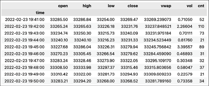
   Figure 2.14: Preview of the DataFrame with time bars

6. Get the tick bars:

   bar_size = 50
   df["tick_group"] = (
       pd.Series(list(range(len(df))))
       .div(bar_size)
       .apply(np.floor)
       .astype(int)
       .values
   )
   df_grouped_ticks = df.groupby("tick_group")
   tick_bars = get_bars(df_grouped_ticks, add_time=True)
   tick_bars
   

   Running the code generates the following tick bars:

   

   Figure 2.15: Preview of the DataFrame with tick bars

   We can see that each group contains exactly 50 trades, just as we intended.

7. Get the volume bars:

   bar_size = 1
   df["cum_qty"] = df["qty"].cumsum()
   df["vol_group"] = (
       df["cum_qty"]
       .div(bar_size)
       .apply(np.floor)
       .astype(int)
       .values
   )
   df_grouped_ticks = df.groupby("vol_group")
   volume_bars = get_bars(df_grouped_ticks, add_time=True)
   volume_bars
   

   Running the code generates the following volume bars:

   

   Figure 2.16: Preview of the DataFrame with volume bars

   We can see that all the bars contain approximately the same volume. The last one is a bit smaller, simply because we did not have enough total volume in the 500 trades.

8. Get the dollar bars:

   bar_size = 50000
   df["cum_value"] = df["quoteQty"].cumsum()
   df["value_group"] = (
       df["cum_value"]
       .div(bar_size)
       .apply(np.floor)
       .astype(int)
       .values
   )
   df_grouped_ticks = df.groupby("value_group")
   dollar_bars = get_bars(df_grouped_ticks, add_time=True)
   dollar_bars
   

   Running the code generates the following dollar bars:

Figure 2.17: Preview of the DataFrame with dollar bars

How it works…

After importing the libraries, we instantiated the Binance client and downloaded the 500 most recent trades in the BTCEUR market using the trades method of the Binance client. We chose this one on purpose, as it is not as popular as BTCUSD and the default 500 trades actually span a few minutes. We could increase the number of trades up to 1,000 using the limit argument.

In Step 3, we prepared the data for further analysis, that is, we converted the response from the Binance client into a pandas DataFrame, dropped two columns we will not be using, converted the time column into datetime, and converted to columns containing prices and quantities into numeric ones, as they were expressed as object type, which is a string.

Then, we defined a helper function for calculating the bars per some group. The input of the function must be a DataFrameGroupBy object, that is, the output of applying the groupby method to a pandas DataFrame. That is because the function calculates a bunch of aggregate statistics:

• OHLC values using the ohlc method.
• The volume-weighted average price (VWAP) by applying the np.average method and using the quantity of the trade as the weights argument.
• The total volume as the sum of the traded quantity.
• The number of trades in a bar by using the size method.
• Optionally, the function also returns the timestamp of the bar, which is simply the last timestamp of the group.

All of those are separate DataFrames, which we ultimately concatenated using the pd.concat function.

In Step 5, we calculated the time bars. We had to use the groupby method combined with pd.Grouper. We indicated we want to create the groups on the time column and used a one-minute frequency. Then, we passed the DataFrameGroupBy object to our get_bars function, which returned the time bars.

In Step 6, we calculated the tick bars. The process was slightly different than with time bars, as we first had to create the column on which we want to group the trades. The idea was that we group the trades in blocks of 50 (this is an arbitrary number and should be determined according to the logic of the analysis). To create such groups, we divided the row number by the chosen bar size, rounded the result down (using np.floor), and converted it into an integer. Then, we grouped the trades using the newly created column and applied the get_bars function.

In Step 7, we calculated the volume bars. The process was quite similar to the tick bars. The difference was in creating the grouping column, which this time was based on the cumulative sum of the traded quantity. We selected the bar size of 1 BTC.

The last step was to calculate the dollar bars. The process was almost identical to the volume bars, but we created the grouping column by applying a cumulative sum to the quoteQty column, instead of the qty one used before.

There’s more…

The list of alternative kinds of bars in this recipe is not exhaustive. For example, De Prado (2018) suggests using imbalance bars, which attempt to sample the data when there is an imbalance of buying/selling activity, as this might imply information asymmetry between market participants. The reasoning behind those bars is market participants either buy or sell large quantities of a given asset, but they do not frequently do both simultaneously. Hence, sampling when imbalance events occur helps to focus on large movements and pay less attention to periods without interesting activity.

See also

• De Prado, M. L. (2018). Advances in Financial Machine Learning. John Wiley & Sons.
• https://github.com/binance/binance-connector-python—the GitHub repo of the library used for connecting to Binance’s API

Summary

In this chapter, we have learned how to preprocess financial time series data. We started by showing how to calculate returns and potentially adjust them for inflation. Then, we covered a few of the popular methods for imputing missing values. Lastly, we explained the different approaches to aggregating trade data and why choosing the correct one matters.

We should always pay significant attention to this step, as we not only want to enhance our model’s performance but also to ensure the validity of any analysis. In the next chapter, we will continue working with the preprocessed data and learn how to create time series visualization.