
9
Modeling Volatility with GARCH Class Models
In Chapter 6, Time Series Analysis and Forecasting, we looked at various approaches to modeling time series. However, models such as ARIMA (Autoregressive Integrated Moving Average) cannot account for volatility that is not constant over time (heteroskedastic). We have already explained that some transformations (such as log or Box-Cox transformations) can be used to adjust for modest changes in volatility, but we would like to go a step further and model it.
In this chapter, we focus on conditional heteroskedasticity, which is a phenomenon caused when an increase in volatility is correlated with a further increase in volatility. An example might help to understand this concept. Imagine the price of an asset going down significantly due to some breaking news related to the company. Such a sudden price drop could trigger certain risk management tools of investment funds, which start selling the stocks as a result of the previous decrease in price. This could result in the price plummeting even further. Conditional heteroskedasticity was also clearly visible in the Investigating stylized facts of asset returns recipe, in which we showed that returns exhibit volatility clustering.
We would like to briefly explain the motivation for this chapter. Volatility is an incredibly important concept in finance. It is synonymous with risk and has many applications in quantitative finance. Firstly, it is used in options pricing, as the Black-Scholes model relies on the volatility of the underlying asset. Secondly, volatility has a significant impact on risk management, where it is used to calculate metrics such as the Value-at-Risk (VaR) of a portfolio, the Sharpe ratio, and many more. Thirdly, volatility is also present in trading. Normally, traders make decisions based on predictions of the assets’ prices either rising or falling. However, we can also trade based on predicting whether there will be movement in any direction, that is, whether there will be volatility. Volatility trading is particularly appealing when certain world events (for example, pandemics) are driving markets to move erratically. An example of a product interesting to volatility traders might be the Volatility Index (VIX), which is based on the movements of the S&P 500 index.
By the end of the chapter, we will have covered a selection of GARCH (Generalized Autoregressive Conditional Heteroskedasticity) models—both univariate and multivariate—which are some of the most popular ways of modeling and forecasting volatility. Knowing the basics, it is quite simple to implement more advanced models. We have already mentioned the importance of volatility in finance. By knowing how to model it, we can use such forecasts to replace the previously used naïve ones in many practical use cases in the fields of risk management or derivatives valuation.
In this chapter, we will cover the following recipes:
- Modeling stock returns’ volatility with ARCH models
- Modeling stock returns’ volatility with GARCH models
- Forecasting volatility using GARCH models
- Multivariate volatility forecasting with the CCC-GARCH model
- Forecasting the conditional covariance matrix using DCC-GARCH
Modeling stock returns’ volatility with ARCH models
In this recipe, we approach the problem of modeling the conditional volatility of stock returns with the Autoregressive Conditional Heteroskedasticity (ARCH) model.
To put it simply, the ARCH model expresses the variance of the error term as a function of past errors. To be a bit more precise, it assumes that the variance of the errors follows an autoregressive model. The entire logic of the ARCH method can be represented by the following equations:
![]()
![]()

The first equation represents the return series as a combination of the expected return μ and the unexpected return ![]() .
. ![]() has white noise properties—the conditional mean equal to zero and the time-varying conditional variance
has white noise properties—the conditional mean equal to zero and the time-varying conditional variance ![]() .
.
Error terms are serially uncorrelated but do not need to be serially independent, as they can exhibit conditional heteroskedasticity.
![]() is also known as the mean-corrected return, error term, innovations, or—most commonly—residuals.
is also known as the mean-corrected return, error term, innovations, or—most commonly—residuals.
In general, ARCH (and GARCH) models should only be fitted to the residuals of some other model applied to the original time series. When estimating volatility models, we can assume different specifications of the mean process, for example:
- A zero-mean process—this implies that the returns are only described by the residuals, for example,

- A constant mean process (
 )
) - Mean estimated using linear models such as AR, ARMA, ARIMA, or the more recent heterogeneous autoregressive (HAR) process
In the second equation, we represent the error series in terms of a stochastic component ![]() and a conditional standard deviation
and a conditional standard deviation ![]() , which governs the typical size of the residuals. The stochastic component can also be interpreted as standardized residuals.
, which governs the typical size of the residuals. The stochastic component can also be interpreted as standardized residuals.
The third equation presents the ARCH formula, where ![]() and
and ![]() . Some important points about the ARCH model include:
. Some important points about the ARCH model include:
- The ARCH model explicitly recognizes the difference between the unconditional and the conditional variance of the time series.
- It models the conditional variance as a function of past residuals (errors) from a mean process.
- It assumes the unconditional variance to be constant over time.
- The ARCH model can be estimated using the ordinary least squares (OLS) method.
- We must specify the number of prior residuals (q) in the model—similarly to the AR model.
- The residuals should look like observations of a discrete white noise—zero-mean and stationary (no trends or seasonal effects, that is, no evident serial correlation).
In the original ARCH notation, as well as in the arch library in Python, the lag hyperparameter is denoted with p. However, we use q as the corresponding symbol, in line with the GARCH notation introduced in the next recipe.
The biggest strength of the ARCH model is that the volatility estimates it produces exhibit excess kurtosis (fat tails as compared to Normal distribution), which is in line with the empirical observations about stock returns. Naturally, there are also weaknesses. The first one is that the model assumes the same effects of positive and negative volatility shocks, which is simply not the case. Secondly, it does not explain variations in volatility. That is why the model is likely to over-forecast volatility, as it is slow to respond to large, isolated shocks in the returns series.
In this recipe, we fit the ARCH(1) model to Google’s daily stock returns from the years 2015 to 2021.
How to do it...
Execute the following steps to fit the ARCH(1) model:
- Import the libraries:
import pandas as pd import yfinance as yf from arch import arch_model - Specify the risky asset and the time horizon:
RISKY_ASSET = "GOOG" START_DATE = "2015-01-01" END_DATE = "2021-12-31" - Download data from Yahoo Finance:
df = yf.download(RISKY_ASSET, start=START_DATE, end=END_DATE, adjusted=True) - Calculate the daily returns:
returns = 100 * df["Adj Close"].pct_change().dropna()
returns.name = "asset_returns"
returns.plot(
    title=f"{RISKY_ASSET} returns: {START_DATE} - {END_DATE}"
)
Running the code generates the following plot:
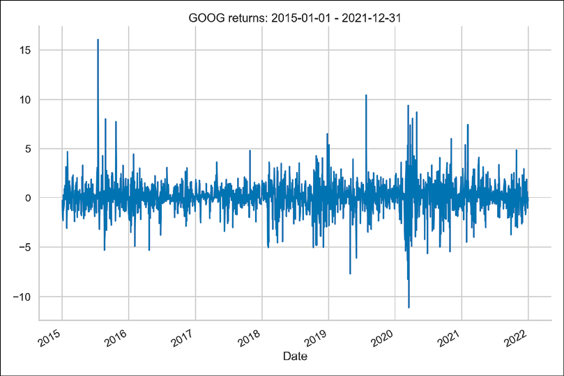
Figure 9.1: Google’s simple returns from the years 2015 to 2021
In the plot, we can observe a few sudden spikes and clear examples of volatility clustering.
- Specify the ARCH model:
model = arch_model(returns, mean="Zero", vol="ARCH", p=1, q=0) - Estimate the model and print the summary:
fitted_model = model.fit(disp="off")
print(fitted_model.summary())
Running the code returns the following summary:
                    Zero Mean - ARCH Model Results
===================================================================
Dep. Variable:      asset_returns   R-squared:                 0.000
Mean Model:         Zero Mean       Adj. R-squared:             .001
Vol Model:          ARCH            Log-Likelihood:         -3302.93
Distribution:       Normal          AIC:                     6609.85
Method:             Maximum         BIC:                     6620.80
                    Likelihood
                                    No. Observations:        1762
Date:           Wed, Jun 08 2022    Df Residuals:            1762
Time:                   22:25:16    Df Model:                0
                        Volatility Model
===================================================================
             coef      std err        t      P>|t|  95.0% Conf. Int.
-------------------------------------------------------------------
omega        1.8625    0.166      11.248  2.359e-29 [ 1.538, 2.187]
alpha[1]     0.3788    0.112       3.374  7.421e-04 [ 0.159, 0.599]
===================================================================
- Plot the residuals and the conditional volatility:
fitted_model.plot(annualize="D")

Figure 9.2: Standardized residuals and the annualized conditional volatility of the fitted ARCH model
We can observe some standardized residuals that are large (in magnitude) and correspond to highly volatile periods.
How it works...
In Steps 2 to 4, we downloaded Google’s daily stock prices and calculated simple returns. When working with ARCH/GARCH models, convergence warnings are likely to occur in the case of very small numbers. This is caused by instabilities in the underlying optimization algorithms of the scipy library. To overcome this issue, we multiplied the returns by 100 to express them as percentages.
In Step 5, we defined the ARCH(1) model. For the mean model, we selected the zero-mean approach, which is suitable for many liquid financial assets. Another viable choice here could be a constant mean. We can use those approaches as opposed to, for example, ARMA models because the serial dependence of the return series might be very limited.
In Step 6, we fitted the model using the fit method. Additionally, we passed disp="off" to the fit method to suppress output from the optimization steps. To fit the model using the arch library, we had to take similar steps to the familiar scikit-learn approach: we first defined the model and then fitted it to the data. One difference would be the fact that with arch, we had to provide the data object while creating the instance of the model, instead of passing it to the fit method as we would have done in scikit-learn. Then, we printed the model’s summary by using the summary method.
In Step 7, we also inspected the standardized residuals and the conditional volatility series by plotting them. The standardized residuals were computed by dividing the residuals by the conditional volatility. We passed annualize="D" to the plot method in order to annualize the conditional volatility series from daily data.
There’s more...
A few more noteworthy points about ARCH models:
- Selecting the zero-mean process is useful when working on residuals from a separately estimated model.
- To detect ARCH effects, we can look at the correlogram of the squared residuals from a certain model (such as the ARIMA model). We need to make sure that the mean of these residuals is equal to zero. We can use the Partial Autocorrelation Function (PACF) plot to infer the value of q, similarly to the approach used in the case of the AR model (please refer to the Modeling time series with ARIMA class models recipe for more details).
- To test the validity of the model, we can inspect whether the standardized residuals and squared standardized residuals exhibit no serial autocorrelation (for example, using the Ljung-Box or Box-Pierce test with the
acorr_ljungboxfunction fromstatsmodels). Alternatively, we can employ the Lagrange Multiplier test (the LM test, also known as Engle’s Test for Autoregressive Conditional Heteroscedasticity) to make sure that the model captures all ARCH effects. To do so, we can use thehet_archfunction fromstatsmodels.
In the following snippet, we test the residuals of the ARCH model with the LM test:
from statsmodels.stats.diagnostic import het_arch
het_arch(fitted_model.resid)
Running the code returns the following tuple:
(98.10927835448403,
 1.3015895084238874e-16,
 10.327662606705564,
 4.2124269229123006e-17)
The first two values in the tuple are the LM test statistic and its corresponding p-value. The latter two are the f-statistic for the F test (an alternative approach to testing for ARCH effects) and its corresponding p-value. We can see that both p-values are below the customary significance level of 0.05, which leads us to reject the null hypothesis stating that the residuals are homoskedastic. This means that the ARCH(1) model fails to capture all ARCH effects in the residuals.
The documentation of the het_arch function suggests that if the residuals are coming from a regression model, we should correct for the number of estimated parameters in that model. For example, if the residuals were coming from an ARMA(2, 1) model, we should pass an additional argument to the het_arch function, ddof = 3, where ddof stands for the degrees of freedom.
See also
Additional resources are available here:
- Engle, R. F. 1982., “Autoregressive conditional heteroscedasticity with estimates of the variance of United Kingdom inflation,” Econometrica, 50(4): 987-1007
Modeling stock returns’ volatility with GARCH models
In this recipe, we present how to work with an extension of the ARCH model, namely the Generalized Autoregressive Conditional Heteroskedasticity (GARCH) model. GARCH can be considered an ARMA model applied to the variance of a time series—the AR component was already expressed in the ARCH model, while GARCH additionally adds the moving average part.
The equation of the GARCH model can be presented as:
![]()
![]()

While the interpretation is very similar to the ARCH model presented in the previous recipe, the difference lies in the last equation, where we can observe an additional component. Parameters are constrained to meet the following: ![]() , and
, and ![]() .
.
In the GARCH model, there are additional constraints on coefficients. For example, in the case of a GARCH(1,1) model, ![]() must be less than 1. Otherwise, the model is unstable.
must be less than 1. Otherwise, the model is unstable.
The two hyperparameters of the GARCH model can be described as:
- p: The number of lag variances
- q: The number of lag residual errors from a mean process
A GARCH(0, q) model is equivalent to an ARCH(q) model.
One way of inferring the lag orders for ARCH/GARCH models is to use the squared residuals from a model used to predict the mean of the original time series. As the residuals are centered around zero, their squares correspond to their variance. We can inspect the ACF/PACF plots of the squared residuals in order to identify patterns in the autocorrelation of the series’ variance (similarly to what we have done to identify the orders of an ARMA/ARIMA model).
In general, the GARCH model shares the strengths and weaknesses of the ARCH model, with the difference that it better captures the effects of past shocks. Please see the There’s more... section to learn about some extensions of the GARCH model that account for the original model’s shortcomings.
In this recipe, we apply the GARCH(1,1) model to the same data as in the previous recipe, in order to clearly highlight the difference between the two modeling approaches.
How to do it...
Execute the following steps to estimate the GARCH(1,1) model in Python:
- Specify the GARCH model:
model = arch_model(returns, mean="Zero", vol="GARCH", p=1, q=1) - Estimate the model and print the summary:
fitted_model = model.fit(disp="off")
print(fitted_model.summary())
Running the code returns the following summary:
                     Zero Mean - GARCH Model Results
====================================================================
Dep. Variable:      asset_returns   R-squared:                 0.000
Mean Model:         Zero Mean       Adj. R-squared:            0.001
Vol Model:          GARCH           Log-Likelihood:         -3246.71
Distribution:       Normal          AIC:                     6499.42
Method:             Maximum         BIC:                     6515.84
                    Likelihood
                                    No. Observations:        1762
Date:           Wed, Jun 08 2022    Df Residuals:            1762
Time:                   22:37:27    Df Model:                0
                          Volatility Model
===================================================================
             coef      std err     t      P>|t|     95.0% Conf. Int.
-------------------------------------------------------------------
omega        0.2864    0.186     1.539   0.124   [-7.844e-02, 0.651]
alpha[1]     0.1697  9.007e-02   1.884 5.962e-02 [-6.879e-03, 0.346]
beta[1]      0.7346    0.128     5.757  8.538e-09    [ 0.485, 0.985]
===================================================================
According to Market Risk Analysis, the usual range of values of the parameters in a stable market would be
 and
and  . However, we should keep in mind that while these ranges will most likely not strictly apply, they already give us some idea of what kinds of values we should be expecting.
We can see that, compared to the ARCH model, the log-likelihood increased, which means that the GARCH model fits the data better. However, we should be cautious when drawing such conclusions. The log-likelihood will most likely increase every time we add more predictors (as we have done with GARCH). In case the number of predictors changes, we should run a likelihood-ratio test in order to compare the goodness-of-fit criteria of two nested regression models.
- Plot the residuals and the conditional volatility:
fitted_model.plot(annualize="D")In the plots below, we can observe the effect of including the extra component (lagged conditional volatility) into the model specification:

Figure 9.3: Standardized residuals and the annualized conditional volatility of the fitted GARCH model
When using ARCH, the conditional volatility series exhibits many spikes, and then immediately returns to a low level. In the case of GARCH, as the model also includes lagged conditional volatility, it takes more time to return to the level observed before the spike.
How it works...
In this recipe, we used the same data as in the previous one to compare the results of the ARCH and GARCH models. For more information on downloading data, please refer to Steps 1 to 4 in the Modeling stock returns’ volatility with ARCH models recipe.
Due to the convenience of the arch library, it was very easy to adjust the code used previously to fit the ARCH model. To estimate the GARCH model, we had to specify the type of volatility model we wanted to use and set an additional argument: q=1.
For comparison’s sake, we left the mean process as a zero-mean process.
There’s more...
In this chapter, we have already used two models to explain and potentially forecast the conditional volatility of a time series. However, there are numerous extensions of the GARCH model, as well as different configurations with which we can experiment in order to find the best-fitting model.
In the GARCH framework, aside from the hyperparameters (such as p and q, in the case of the vanilla GARCH model), we can modify the models described next.
Conditional mean model
As explained before, we apply the GARCH class models to residuals obtained after fitting another model to the series. Some popular choices for the mean model are:
- Zero-mean
- Constant mean
- Any variant of the ARIMA model (including potential seasonality adjustment, as well as external regressors)—some popular choices in the literature are ARMA or even AR models
- Regression models
We should be aware of one thing when modeling the conditional mean. For example, we may first fit an ARMA model to our time series and then fit a GARCH model to the residuals of the first model. However, this is not the preferred way. That is because, in general, the ARMA estimates will be inconsistent (or consistent but inefficient, in the case when there are only AR terms and no MA terms), which will also impact the following GARCH estimates. The inconsistency arises because the first model (ARMA/ARIMA) assumes conditional homoskedasticity, while we are explicitly modeling conditional heteroskedasticity with the GARCH model in the second step. That is why the preferred way is to estimate both models simultaneously, for example, using the arch library (or the rugarch package for R).
Conditional volatility model
There are numerous extensions to the GARCH framework. Some popular models include:
- GJR-GARCH: A variant of the GARCH model that takes into account the asymmetry of the returns (negative returns tend to have a stronger impact on volatility than positive ones)
- EGARCH: Exponential GARCH
- TGARCH: Threshold GARCH
- FIGARCH: Fractionally integrated GARCH, used with non-stationary data
- GARCH-MIDAS: In this class of models, volatility is decomposed into a short-term GARCH component and a long-term component driven by an additional explanatory variable
- Multivariate GARCH models, such as CCC-/DCC-GARCH
The first three models use slightly different approaches to introduce asymmetry into the conditional volatility specification. This is in line with the belief that negative shocks have a stronger impact on volatility than positive shocks.
Distribution of errors
In the Investigating stylized facts of asset returns recipe, we saw that the distribution of returns is not Normal (skewed, with heavy tails). That is why distributions other than Gaussian might be more fitting for errors in the GARCH model.
Some possible choices are:
- Student’s t-distribution
- Skew-t distribution (Hansen, 1994)
- Generalized Error Distribution (GED)
- Skewed Generalized Error Distribution (SGED)
The arch library not only provides most of the models and distributions mentioned above, but it also allows for the use of your own volatility models/distributions of errors (as long as they fit into a predefined format). For more information on this, please refer to the excellent documentation.
See also
Additional resources are available here:
- Alexander, C. 2008. Market Risk Analysis, Practical Financial Econometrics (Vol. 2). John Wiley & Sons.
- Bollerslev, T., 1986. “Generalized Autoregressive Conditional Heteroskedasticity. Journal of Econometrics, 31, (3): 307–327. : https://doi.org/10.1016/0304-4076(86)90063-1
- Glosten, L. R., Jagannathan, R., and Runkle, D. E., 1993. “On the relation between the expected value and the volatility of the nominal excess return on stocks,” The Journal of Finance, 48 (5): 1779–1801: https://doi.org/10.1111/j.1540-6261.1993.tb05128.x
- Hansen, B. E., 1994. “Autoregressive conditional density estimation,” International Economic Review, 35(3): 705–730: https://doi.org/10.2307/2527081
- Documentation of the
archlibrary—https://arch.readthedocs.io/en/latest/index.html
Forecasting volatility using GARCH models
In the previous recipes, we have seen how to fit ARCH/GARCH models to a return series. However, the most interesting/relevant case of using ARCH class models would be to forecast the future values of the volatility.
There are three approaches to forecasting volatility using GARCH class models:
- Analytical — due to the inherent structure of ARCH class models, analytical forecasts are always available for the one step-ahead forecast. Multi-step analytical forecasts can be obtained using a forward recursion; however, that is only possible for models that are linear in the square of the residuals (such as GARCH or Heterogeneous ARCH).
- Simulation—simulation-based forecasts use the structure of an ARCH class model to forward simulate possible volatility paths using the assumed distribution of residuals. In other words, they use random number generators (assuming specific distributions) to draw the standardized residuals. This approach creates x possible volatility paths and then produces the average as the final forecast. Simulation-based forecasts are always available for any horizon. As the number of simulations increases toward infinity, the simulation-based forecasts will converge to the analytical forecasts.
- Bootstrap (also known as the Filtered Historical Simulation)—those forecasts are very similar to the simulation-based forecasts with the difference that they generate (to be precise, draw with replacement) the standardized residuals using the actual input data and the estimated parameters. This approach requires a minimal amount of in-sample data to use prior to producing the forecasts.
Due to the specification of ARCH class models, the first out-of-sample forecast will always be fixed, regardless of which approach we use.
In this recipe, we fit a GARCH(1,1) model with Student’s t distributed residuals to Microsoft’s stock returns from the years 2015 to 2020. Then, we create 3-step ahead forecasts for each day of 2021.
How to do it...
Execute the following steps to create 3-step ahead volatility forecasts using a GARCH model:
- Import the libraries:
import pandas as pd import yfinance as yf from datetime import datetime from arch import arch_model - Download data from Yahoo Finance and calculate simple returns:
df = yf.download("MSFT", start="2015-01-01", end="2021-12-31", adjusted=True) returns = 100 * df["Adj Close"].pct_change().dropna() returns.name = "asset_returns" - Specify the GARCH model:
model = arch_model(returns, mean="Zero", vol="GARCH", dist="t", p=1, q=1) - Define the split date and fit the model:
SPLIT_DATE = datetime(2021, 1, 1) fitted_model = model.fit(last_obs=SPLIT_DATE, disp="off") - Create and inspect the analytical forecasts:
forecasts_analytical = fitted_model.forecast(horizon=3,
                                             start=SPLIT_DATE,
                                             reindex=False)
forecasts_analytical.variance.plot(
    title="Analytical forecasts for different horizons"
)
Running the snippet generates the following plot:

Figure 9.4: Analytical forecasts for horizons 1, 2, and 3
Using the snippet below, we can inspect the generated forecasts.
forecasts_analytical.variance
Figure 9.5: Table presenting the analytical forecasts for horizons 1, 2, and 3
Each column contains the h-step ahead forecasts generated on the date indicated by the index. When the forecasts are created, the date from the
Datecolumn corresponds to the last data point used to generate the forecasts. For example, the columns with the date 2021-01-08 contain the forecasts for January 9, 10, and 11. Those forecasts were created using data up to and including January 8.
- Create and inspect the simulation forecasts:
forecasts_simulation = fitted_model.forecast(
    horizon=3,
    start=SPLIT_DATE,
    method="simulation",
    reindex=False
)

forecasts_simulation.variance.plot(
    title="Simulation forecasts for different horizons"
)
Running the snippet generates the following plot:

Figure 9.6: Simulation-based forecasts for horizons 1, 2, and 3
- Create and inspect the bootstrap forecasts:
forecasts_bootstrap = fitted_model.forecast(horizon=3,
                                            start=SPLIT_DATE,
                                            method="bootstrap",
                                            reindex=False)
forecasts_bootstrap.variance.plot(
    title="Bootstrap forecasts for different horizons"
)
Running the snippet generates the following plot:

Figure 9.7: Bootstrap-based forecasts for horizons 1, 2, and 3
Inspecting the three plots leads to the conclusion that the shape of the volatility forecasts from the three different methods is very similar.
How it works...
In the first two steps, we imported the required libraries and downloaded Microsoft’s stock prices from the years 2015 to 2021. We calculated the simple returns and multiplied the values by 100 to avoid potential convergence issues during optimization.
In Step 3, we specified our GARCH model, that is, a zero-mean GARCH(1, 1) with residuals following Student’s t distribution.
In Step 4, we defined a date (a datetime object) used for splitting the training and test sets. Then, we fitted the model using the fit method. This time, we specified the last_obs argument to indicate when the training set ends. We passed in the value of datetime(2021, 1, 1), which means that the last observation actually used for training would be the last date of December 2020.
In Step 5, we created the analytical forecasts using the forecast method of a fitted GARCH model. We specified the forecast horizon and the start date (which is the same as the last_obs, which we provided when fitting the model). Then, we plotted the forecasts for each horizon.
In general, using the forecast method returns an ARCHModelForecast object with 4 main attributes that we might find useful:
mean—the forecast of the conditional meanvariance—the forecast of the conditional variance of the processresidual_variance—the forecast of the residual variance. These values will differ from the ones stored invariance(for horizons larger than 1) whenever the model has mean dynamics, for example, an AR process.simulations—an object containing the individual simulations (only for the simulation and bootstrap approaches) used for generating the forecasts.
In Steps 6 and 7, we generated the analogical 3-step ahead forecasts using the simulation and bootstrap methods. We only added the optional method argument to the forecast method to indicate which forecasting approach we would like to use. By default, those methods use 1,000 simulations to create the forecasts, but we can change this number to our liking.
There’s more...
We can quite easily visually compare the differences in the forecasts obtained using various forecasting approaches. In this case, we would like to compare the analytical and bootstrap approaches over 2020. We chose 2020 as this was the last year used in the training sample.
Execute the following steps to compare 10-step ahead volatility forecasts over the year 2020:
- Import the libraries:
import numpy as np - Estimate the 10-step ahead volatility forecasts for 2020 using the analytical and bootstrap approaches:
FCST_HORIZON = 10
vol_analytic = (
    fitted_model.forecast(horizon=FCST_HORIZON,
                          start=datetime(2020, 1, 1),
                          reindex=False)
    .residual_variance["2020"]
    .apply(np.sqrt)
)
vol_bootstrap = (
    fitted_model.forecast(horizon=FCST_HORIZON,
                          start=datetime(2020, 1, 1),
                          method="bootstrap",
                          reindex=False)
    .residual_variance["2020"]
    .apply(np.sqrt)
)
While creating the forecasts, we changed the horizon and the start date. We recovered the residual variance from the fitted models, filtered for the forecasts made in 2020, and then took the square root to convert the variance into volatility.
- Get the conditional volatility for 2020:
vol = fitted_model.conditional_volatility["2020"] - Create the hedgehog plot:
ax = vol.plot(
    title="Comparison of analytical vs bootstrap volatility forecasts",
    alpha=0.5
)
ind = vol.index
for i in range(0, 240, 10):
    vol_a = vol_analytic.iloc[i]
    vol_b = vol_bootstrap.iloc[i]
    start_loc = ind.get_loc(vol_a.name)
    new_ind = ind[(start_loc+1):(start_loc+FCST_HORIZON+1)]
    vol_a.index = new_ind
    vol_b.index = new_ind
    ax.plot(vol_a, color="r")
    ax.plot(vol_b, color="g")

labels = ["Volatility", "Analytical Forecast",
          "Bootstrap Forecast"]
legend = ax.legend(labels)

Figure 9.8: Comparison of analytical and bootstrap-based approaches to volatility forecasting
A hedgehog plot is a useful kind of visualization for showing the differences between the two forecasting approaches over a longer period of time. In this case, we plotted the 10-step ahead forecasts every 10 days.
What is interesting to note is the peak in volatility that occurred in March 2020. We can see that close to the peak, the GARCH model is predicting a decrease in volatility over the next few days. To get a better understanding of how that forecast was created, we can refer to the underlying data. By inspecting the DataFrames containing the observed volatility and the forecasts, we can state that the peak happened on March 17, while the plotted forecast was created using data up until March 16.
When inspecting a single volatility model at a time, it might be easier to use the hedgehog_plot method of the fitted arch_model to create a similar plot.
Multivariate volatility forecasting with the CCC-GARCH model
In this chapter, we have already considered multiple univariate conditional volatility models. That is why, in this recipe, we move to the multivariate setting. As a starting point, we consider Bollerslev’s Constant Conditional Correlation GARCH (CCC-GARCH) model. The idea behind it is quite simple. The model consists of N univariate GARCH models, related to each other via a constant conditional correlation matrix R.
Like before, we start with the model’s specification:
![]()
![]()
![]()
In the first equation, we represent the return series. The key difference between this representation and the one presented in previous recipes is the fact that this time, we are considering multivariate returns. That is why rt is actually a vector of returns rt = (r1t, …, rnt). The mean and error terms are represented analogically. To highlight this, we use bold font when considering vectors or matrices.
The second equation shows that the error terms come from a Multivariate Normal distribution with zero means and a conditional covariance matrix ![]() (of size N x N).
(of size N x N).
The elements of the conditional covariance matrix are defined as:
- Diagonal:

- Off-diagonal:

The third equation presents the decomposition of the conditional covariance matrix. Dt represents a matrix containing the conditional standard deviations on the diagonal, and R is a correlation matrix.
The key ideas of the model are as follows:
- The model avoids the problem of guaranteeing positive definiteness of
 by splitting it into variances and correlations.
 - The conditional correlations between error terms are constant over time.
- Individual conditional variances follow a univariate GARCH(1,1) model.
In this recipe, we estimate the CCC-GARCH model on a series of stock returns for three US tech companies. For more details about the estimation of the CCC-GARCH model, please refer to the How it works... section.
How to do it...
Execute the following steps to estimate the CCC-GARCH model in Python:
- Import the libraries:
import pandas as pd import numpy as np import yfinance as yf from arch import arch_model - Specify the risky assets and the time horizon:
RISKY_ASSETS = ["GOOG", "MSFT", "AAPL"] START_DATE = "2015-01-01" END_DATE = "2021-12-31" - Download data from Yahoo Finance:
df = yf.download(RISKY_ASSETS, start=START_DATE, end=END_DATE, adjusted=True) - Calculate the daily returns:
returns = 100 * df["Adj Close"].pct_change().dropna()
returns.plot(
    subplots=True,
    title=f"Stock returns: {START_DATE} - {END_DATE}"
)
Running the snippet generates the following plot:

Figure 9.9: Simple returns of Apple, Google, and Microsoft
- Define lists for storing objects:
coeffs = [] cond_vol = [] std_resids = [] models = [] - Estimate the univariate GARCH models:
for asset in returns.columns: model = arch_model(returns[asset], mean="Constant", vol="GARCH", p=1, q=1) model = model.fit(update_freq=0, disp="off"); coeffs.append(model.params) cond_vol.append(model.conditional_volatility) std_resids.append(model.std_resid) models.append(model) - Store the results in DataFrames:
coeffs_df = pd.DataFrame(coeffs, index=returns.columns)
cond_vol_df = (
    pd.DataFrame(cond_vol)
    .transpose()
    .set_axis(returns.columns,
              axis="columns")
)
std_resids_df = (
    pd.DataFrame(std_resids)
    .transpose()
    .set_axis(returns.columns
              axis="columns")
)
The following table contains the estimated coefficients for each return series:

Figure 9.10: Coefficients of the estimated univariate GARCH models
- Calculate the constant conditional correlation matrix (R):
R = ( std_resids_df .transpose() .dot(std_resids_df) .div(len(std_resids_df)) ) - Calculate the one-step ahead forecast of the conditional covariance matrix:
# define objects
diag = []
D = np.zeros((len(RISKY_ASSETS), len(RISKY_ASSETS)))

# populate the list with conditional variances
for model in models:
    diag.append(model.forecast(horizon=1).variance.iloc[-1, 0])
# take the square root to obtain volatility from variance
diag = np.sqrt(diag)
# fill the diagonal of D with values from diag
np.fill_diagonal(D, diag)

# calculate the conditional covariance matrix
H = np.matmul(np.matmul(D, R.values), D)
The calculated one-step ahead forecast looks as follows:
array([[2.39962391, 1.00627878, 1.19839517],
       [1.00627878, 1.51608369, 1.12048865],
       [1.19839517, 1.12048865, 1.87399738]])
We can compare this matrix to the one obtained using a more complex DCC-GARCH model, which we cover in the next recipe.
How it works...
In Steps 2 and Step 3, we downloaded the daily stock prices of Google, Microsoft, and Apple. Then, we calculated simple returns and multiplied them by 100 to avoid encountering convergence errors.
In Step 5, we defined empty lists for storing elements required at later stages: GARCH coefficients, conditional volatilities, standardized residuals, and the models themselves (used for forecasting).
In Step 6, we iterated over the columns of the DataFrame containing the stock returns and fitted a univariate GARCH model to each of the series. We stored the results in the predefined lists. Then, we wrangled the data in order to have objects such as residuals in DataFrames, to make working with them easier.
In Step 8, we calculated the constant conditional correlation matrix (R) as the unconditional correlation matrix of zt:

Here, zt stands for time t standardized residuals from the univariate GARCH models.
In the last step, we obtained one-step ahead forecasts of the conditional covariance matrix Ht+1. To do so, we did the following:
- We created a matrix Dt+1 of zeros, using
np.zeros. - We stored the one-step ahead forecasts of conditional variances from univariate GARCH models in a list called
diag. - Using
np.fill_diagonal, we placed the elements of the list calleddiagon the diagonal of the matrix Dt+1 - Following equation 3 from the introduction, we obtained the one-step ahead forecast using matrix multiplication (
np.matmul).
See also
Additional resources are available here:
- Bollerslev, T.1990. “Modeling the Coherence in Short-Run Nominal Exchange Rates: A Multivariate Generalized ARCH Approach,” Review of Economics and Statistics, 72(3): 498–505: https://doi.org/10.2307/2109358
Forecasting the conditional covariance matrix using DCC-GARCH
In this recipe, we cover an extension of the CCC-GARCH model: Engle’s Dynamic Conditional Correlation GARCH (DCC-GARCH) model. The main difference between the two is that in the latter, the conditional correlation matrix is not constant over time—we work with Rt instead of R.
There are some nuances in terms of estimation, but the outline is similar to the CCC-GARCH model:
- Estimate the univariate GARCH models for conditional volatility
- Estimate the DCC model for conditional correlations
In the second step of estimating the DCC model, we use a new matrix Qt, representing a proxy correlation process.
![]()
![]()
![]()
The first equation describes the relationship between the conditional correlation matrix Rt and the proxy process Qt. The second equation represents the dynamics of the proxy process. The last equation shows the definition of ![]() , which is defined as the unconditional correlation matrix of standardized residuals from the univariate GARCH models.
, which is defined as the unconditional correlation matrix of standardized residuals from the univariate GARCH models.
This representation of the DCC model uses an approach called correlation targeting. It means that we are effectively reducing the number of parameters we need to estimate to two: ![]() and
and ![]() . This is similar to volatility targeting in the case of univariate GARCH models, further described in the There’s more... section.
. This is similar to volatility targeting in the case of univariate GARCH models, further described in the There’s more... section.
At the time of writing, there is no Python library that we can use to estimate DCC-GARCH models. One solution would be to write such a library from scratch. Another, more time-efficient solution would be to use a well-established R package for that task. That is why in this recipe, we also introduce how to efficiently make Python and R work together in one Jupyter notebook (this can also be done in a normal .py script). The rpy2 library is an interface between both languages. It enables us to not only run both R and Python in the same notebook but also to transfer objects between the two environments.
In this recipe, we use the same data as in the previous one, in order to highlight the differences in the approach and results.
Getting ready
For details on how to easily install R, please refer to the following resources:
If you use conda as your package manager, the process of setting everything up can be greatly simplified. If you just install rpy2 using the conda install rpy2 command, the package manager will automatically install the latest version of R and some other required dependencies.
Before executing the following code, please make sure to run the code from the previous recipe to have the data available.
How to do it...
Execute the following steps to estimate a DCC-GARCH model in Python (using R):
- Set up the connection between Python and R using
rpy2:%load_ext rpy2.ipython - Install the
rmgarchR package and load it:%%R install.packages('rmgarch', repos = "http://cran.us.r-project.org") library(rmgarch)We only need to install the
rmgarchpackage once. After doing so, you can safely comment out the line starting withinstall.packages.
- Import the dataset into R:
%%R -i returns
print(head(returns))
Using the preceding command, we print the first five rows of the R
data.frame:AAPL GOOG MSFT 2015-01-02 00:00:00 -0.951253138 -0.3020489 0.6673615 2015-01-05 00:00:00 -2.817148406 -2.0845731 -0.9195739 2015-01-06 00:00:00 0.009416247 -2.3177049 -1.4677364 2015-01-07 00:00:00 1.402220689 -0.1713264 1.2705295 2015-01-08 00:00:00 3.842214047 0.3153082 2.9418228
- Define the model specification:
%%R # define GARCH(1,1) model univariate_spec <- ugarchspec( mean.model = list(armaOrder = c(0,0)), variance.model = list(garchOrder = c(1,1), model = "sGARCH"), distribution.model = "norm" ) # define DCC(1,1) model n <- dim(returns)[2] dcc_spec <- dccspec( uspec = multispec(replicate(n, univariate_spec)), dccOrder = c(1,1), distribution = "mvnorm" ) - Estimate the model:
%%R
dcc_fit <- dccfit(dcc_spec, data=returns)
dcc_fit
The following table contains the model’s specification summary, estimated coefficients, as well as a selection of goodness-of-fit criteria:
*---------------------------------*
*          DCC GARCH Fit          *
*---------------------------------*
Distribution         :  mvnorm
Model                :  DCC(1,1)
No. Parameters       :  17
[VAR GARCH DCC UncQ] : [0+12+2+3]
No. Series           :  3
No. Obs.             :  1762
Log-Likelihood       :  -8818.787
Av.Log-Likelihood    :  -5
Optimal Parameters
--------------------------------------------------------------------
               Estimate  Std. Error  t value Pr(>|t|)
[AAPL].mu      0.189285    0.037040   5.1102 0.000000
[AAPL].omega   0.176370    0.051204   3.4445 0.000572
[AAPL].alpha1  0.134726    0.026084   5.1651 0.000000
[AAPL].beta1   0.811601    0.029763  27.2691 0.000000
[GOOG].mu      0.125177    0.040152   3.1176 0.001823
[GOOG].omega   0.305000    0.163809   1.8619 0.062614
[GOOG].alpha1  0.183387    0.089046   2.0595 0.039449
[GOOG].beta1   0.715766    0.112531   6.3606 0.000000
[MSFT].mu      0.149371    0.030686   4.8677 0.000001
[MSFT].omega   0.269463    0.086732   3.1068 0.001891
[MSFT].alpha1  0.214566    0.052722   4.0698 0.000047
[MSFT].beta1   0.698830    0.055597  12.5695 0.000000
[Joint]dcca1   0.060145    0.016934   3.5518 0.000383
[Joint]dccb1   0.793072    0.059999  13.2180 0.000000
Information Criteria
---------------------

Akaike       10.029
Bayes        10.082
Shibata      10.029
Hannan-Quinn 10.049
- Calculate the five-step ahead forecasts:
forecasts <- dccforecast(dcc_fit, n.ahead = 5) - Access the forecasts:
%%R

# conditional covariance matrix
forecasts@mforecast$H
# conditional correlation matrix
forecasts@mforecast$R
# proxy correlation process
forecasts@mforecast$Q
# conditional mean forecasts
forecasts@mforecast$mu
The following image shows the five-step ahead forecasts of the conditional covariance matrix:
[[1]]
, , 1

         [,1]     [,2]     [,3]
[1,] 2.397337 1.086898 1.337702
[2,] 1.086898 1.515434 1.145010
[3,] 1.337702 1.145010 1.874023

, , 2

         [,1]     [,2]     [,3]
[1,] 2.445035 1.138809 1.367728
[2,] 1.138809 1.667607 1.231062
[3,] 1.367728 1.231062 1.981190

, , 3

         [,1]     [,2]     [,3]
[1,] 2.490173 1.184169 1.395189
[2,] 1.184169 1.804434 1.308254
[3,] 1.395189 1.308254 2.079076
, , 4
         [,1]     [,2]     [,3]
[1,] 2.532888 1.224255 1.420526
[2,] 1.224255 1.927462 1.377669
[3,] 1.420526 1.377669 2.168484

, , 5

         [,1]     [,2]     [,3]
[1,] 2.573311 1.259997 1.444060
[2,] 1.259997 2.038083 1.440206
[3,] 1.444060 1.440206 2.250150
We can now compare this forecast (the first step) to the one obtained using a simpler CCC-GARCH model. The values of the one-step ahead conditional covariance forecasts are very similar for CCC- and DCC-GARCH models.
How it works...
In this recipe, we used the same data as in the previous recipe, in order to compare the results of the CCC- and DCC-GARCH models. For more information on downloading the data, please refer to Steps 1 to 4 in the previous recipe.
To work with Python and R at the same time, we used the rpy2 library. In this recipe, we presented how to use the library in combination with Jupyter Notebook. For more details on how to use the library in a .py script, please refer to the official documentation. Also, we do not delve into the details of R code in general, as this is outside the scope of this book.
In Step 1, aside from loading any libraries, we also had to use the following magic command: %load_ext rpy2.ipython. It enabled us to run R code by adding %%R to the beginning of a cell in the Notebook. For that reason, please assume that any code block in this chapter is a separate Notebook cell (see the Jupyter Notebook in the accompanying GitHub repository for more information).
In Step 2, we had to install the required R dependencies. To do so, we used the install.packages function, and we specified the repository we wanted to use.
In Step 3, we moved the pandas DataFrame into the R environment. To do so, we passed the extra code -i returns, together with the %%R magic command. We could have imported the data in any of the ensuing steps.
When you want to move a Python object to R, do some manipulation/modeling, and move the final results back to Python, you can use the following syntax: %%R -i input_object -o output_object.
In Step 4, we defined the DCC-GARCH model’s specification. First, we defined the univariate GARCH specification (for conditional volatility estimation) using ugarchspec. This function comes from a package called rugarch, which is the framework for univariate GARCH modeling. By not specifying the ARMA parameters, we chose a constant mean model. For the volatility, we used a GARCH(1,1) model with normally distributed innovations. Secondly, we also specified the DCC model. To do so, we:
- Replicated the univariate specification for each returns series – in this case, three
- Specified the order of the DCC model—in this case, DCC(1,1)
- Specified the multivariate distribution—in this case, Multivariate Normal
We could see the summary of the specification by calling the dcc_spec object.
In Step 5, we estimated the model by calling the dccfit function with the specification and data as arguments. Afterward, we obtained five-step ahead forecasts by using the dccforecast function, which returned nested objects such as:
H: the conditional covariance matrixR: the conditional correlation matrixQ: the proxy process for the correlation matrixmu: the conditional mean
Each one of them contained five-step ahead forecasts, stored in lists.
There’s more...
In this section, we would also like to go over a few more details on estimating GARCH models.
Estimation details
In the first step of estimating the DCC-GARCH model, we can additionally use an approach called variance targeting. The idea is to reduce the number of parameters we need to estimate in the GARCH model.
To do so, we can slightly modify the GARCH equation. The original equation runs as follows:

Unconditional volatility is defined as:
![]()
We can now plug it into the GARCH equation and produce the following:

In the last step, we replace the unconditional volatility with the sample variance of the returns:
By doing so, we have one less parameter to estimate for each GARCH equation. Also, the unconditional variance implied by the model is guaranteed to be equal to the unconditional sample variance. To use variance targeting in practice, we add an extra argument to the ugarchspec function call: ugarchspec(..., variance.targeting = TRUE).
Univariate and multivariate GARCH models
It is also worth mentioning that rugarch and rmgarch work nicely together, as they were both developed by the same author and created as a single go-to framework for estimating GARCH models in R. We have already gained some experience with this when we used the ugarchspec function in the first step of estimating the DCC-GARCH model. There is much more to discover in terms of that package.
Parallelizing the estimation of multivariate GARCH models
Lastly, the estimation process of the DCC-GARCH model can be easily parallelized, with the help of the parallel R package.
To potentially speed up computations with parallelization, we reused the majority of the code from this recipe and added a few extra lines. First, we had to set up a cluster by using makePSOCKcluster from the parallel package and indicated that we would like to use three cores. Then, we defined the parallelizable specification using multifit. Lastly, we fitted the DCC-GARCH model. The difference here, compared to the previously used code, is that we additionally passed the fit and cluster arguments to the function call. When we are done with the estimation, we stop the cluster. You can find the entire snippet below:
%%R
# parallelized DCC-GARCH(1,1)
library("parallel")
# set up the cluster
cl <- makePSOCKcluster(3)
# define parallelizable specification
parallel_fit <- multifit(multispec(replicate(n, univariate_spec)),
                         returns,
                         cluster = cl)
# fit the DCC-GARCH model
dcc_fit <- dccfit(dcc_spec,
                  data = returns,
                  fit.control = list(eval.se = TRUE),
                  fit = parallel_fit,
                  cluster = cl)
# stop the cluster
stopCluster(cl)
Using the preceding code, we can significantly speed up the estimation of the DCC-GARCH model. The improvement in performance is mostly visible when dealing with large volumes of data. Also, the approach of using the parallel package together with multifit can be used to speed up the calculations of various GARCH and ARIMA models from the rugarch and rmgarch packages.
See also
Additional resources:
- Engle, R.F., 2002. “Dynamic Conditional Correlation: A Simple Class of Multivariate Generalized Autoregressive Conditional Heteroskedasticity Models,” Journal of Business and Economic Statistics, 20(3): 339–350: https://doi.org/10.1198/073500102288618487
- Ghalanos, A. (2019). The
rmgarchmodels: Background and properties. (Version 1.3–0): https://cran.r-project.org/web/packages/rmgarch/vignettes/The_rmgarch_models.pdf rpy2's documentation: https://rpy2.github.io/
Summary
Volatility modeling and forecasting have attracted significant attention in recent years, largely due to their importance in financial markets. In this chapter, we have covered the practical application of GARCH models (both univariate and multivariate) to volatility forecasting. By knowing how to model volatility using GARCH class models, we can use more accurate volatility forecasts to replace the naïve estimates in many practical use cases, for example, risk management, volatility trading, and derivatives valuation.
We have focused on GARCH models due to their ability to capture volatility clustering. However, there are other approaches to volatility modeling. For example, regime-switching models assume that there are certain repeating patterns (regimes) in data. Therefore, we should be able to predict future states by using parameter estimates based on past observations.