1
Acquiring Financial Data
The first chapter of this book is dedicated to a very important (some may say the most important) part of any data science/quantitative finance project—gathering data. In line with the famous adage “garbage in, garbage out,” we should strive to obtain data of the highest possible quality and then correctly preprocess it for later use with statistical and machine learning algorithms. The reason for this is simple—the results of our analyses are highly dependent on the input data and no sophisticated model will be able to compensate for that. That is also why in our analyses, we should be able to use our (or someone else’s) understanding of the economic/financial domain to motivate certain data for, for example, modeling stock returns.
One of the most frequently reported issues among the readers of the first edition of this book was getting high-quality data. That is why in this chapter we spend more time exploring different sources of financial data. While quite a few of these vendors offer similar information (prices, fundamentals, and so on), they also offer additional, unique data that can be downloaded via their APIs. An example could be company-related news articles or pre-computed technical indicators. That is why we will download different types of data depending on the recipe. However, be sure to inspect the documentation of the library/API, as most likely its vendor also provides standard data such as prices.
Additional examples are also covered in the Jupyter notebooks, which you can find in the accompanying GitHub repository.
The data sources in this chapter were selected intentionally not only to showcase how easy it can be to gather high-quality data using Python libraries but also to show that the gathered data comes in many shapes and sizes.
Sometimes we will get a nicely formatted pandas DataFrame, while other times it might be in JSON format or even bytes that need to be processed and then loaded as a CSV. Hopefully, these recipes will sufficiently prepare you to work with any kind of data you might encounter online.
Something to bear in mind while reading this chapter is that data differs among sources. This means that the prices we downloaded from two vendors will most likely differ, as those vendors also get their data from different sources and might use other methods to adjust the prices for corporate actions. The best practice is to find a source you trust the most concerning a particular type of data (based on, for example, opinion on the internet) and then use it to download the data you need. One additional thing to keep in mind is that when building algorithmic trading strategies, the data we use for modeling should align with the live data feed used for executing the trades.
This chapter does not cover one important type of data—alternative data. This could be any type of data that can be used to generate some insights into predicting asset prices. Alternative data can include satellite images (for example, tracking shipping routes, or the development of a certain area), sensor data, web traffic data, customer reviews, etc. While there are many vendors specializing in alternative data (for example, Quandl/Nasdaq Data Link), you can also get some by accessing publicly available information via web scraping. As an example, you could scrape customer reviews from Amazon or Yelp. However, those are often bigger projects and are unfortunately outside of the scope of this book. Also, you need to make sure that web scraping a particular website is not against its terms and conditions!
Using the vendors mentioned in this chapter, you can get quite a lot of information for free. But most of those providers also offer paid tiers. Remember to do thorough research on what the data suppliers actually provide and what your needs are before signing up for any of the services.
In this chapter, we cover the following recipes:
- Getting data from Yahoo Finance
- Getting data from Nasdaq Data Link
- Getting data from Intrinio
- Getting data from Alpha Vantage
- Getting data from CoinGecko
Getting data from Yahoo Finance
One of the most popular sources of free financial data is Yahoo Finance. It contains not only historical and current stock prices in different frequencies (daily, weekly, and monthly), but also calculated metrics, such as the beta (a measure of the volatility of an individual asset in comparison to the volatility of the entire market), fundamentals, earnings information/calendars, and many more.
For a long period of time, the go-to tool for downloading data from Yahoo Finance was the pandas-datareader library. The goal of the library was to extract data from a variety of sources and store it in the form of a pandas DataFrame. However, after some changes to the Yahoo Finance API, this functionality was deprecated. It is definitely good to be familiar with this library, as it facilitates downloading data from sources such as FRED (Federal Reserve Economic Data), the Fama/French Data Library, or the World Bank. Those might come in handy for different kinds of analyses and some of them are presented in the following chapters.
As of now, the easiest and fastest way of downloading historical stock prices is to use the yfinance library (formerly known as fix_yahoo_finance).
For the sake of this recipe, we are interested in downloading Apple’s stock prices from the years 2011 to 2021.
How to do it…
Execute the following steps to download data from Yahoo Finance:
- Import the libraries:
import pandas as pd import yfinance as yf - Download the data:
df = yf.download("AAPL", start="2011-01-01", end="2021-12-31", progress=False) - Inspect the downloaded data:
print(f"Downloaded {len(df)} rows of data.")
df
Running the code generates the following preview of the DataFrame:

Figure 1.1: Preview of the DataFrame with downloaded stock prices
The result of the request is a pandas DataFrame (2,769 rows) containing daily Open, High, Low, and Close (OHLC) prices, as well as the adjusted close price and volume.
Yahoo Finance automatically adjusts the close price for stock splits, that is, when a company divides the existing shares of its stock into multiple new shares, most frequently to boost the stock’s liquidity. The adjusted close price takes into account not only splits but also dividends.
How it works…
The download function is very intuitive. In the most basic case, we just need to provide the ticker (symbol), and it will try to download all available data since 1950.
In the preceding example, we downloaded daily data from a specific range (2011 to 2021).
Some additional features of the download function are:
- We can download information for multiple tickers at once by providing a list of tickers (
["AAPL", "MSFT"]) or multiple tickers as a string ("AAPL MSFT"). - We can set
auto_adjust=Trueto download only the adjusted prices. - We can additionally download dividends and stock splits by setting
actions='inline'. Those actions can also be used to manually adjust the prices or for other analyses. - Specifying
progress=Falsedisables the progress bar. - The
intervalargument can be used to download data in different frequencies. We could also download intraday data as long as the requested period is shorter than 60 days.
There’s more…
yfinance also offers an alternative way of downloading the data—via the Ticker class. First, we need to instantiate the object of the class:
aapl_data = yf.Ticker("AAPL")
To download the historical price data, we can use the history method:
aapl_data.history()
By default, the method downloads the last month of data. We can use the same arguments as in the download function to specify the range and frequency.
The main benefit of using the Ticker class is that we can download much more information than just the prices. Some of the available methods include:
info—outputs a JSON object containing detailed information about the stock and its company, for example, the company’s full name, a short business summary, which exchange it is listed on, as well as a selection of financial metrics such as the beta coefficientactions—outputs corporate actions such as dividends and splitsmajor_holders—presents the names of the major holdersinstitutional_holders—shows the institutional holderscalendar—shows the incoming events, such as the quarterly earningsearnings/quarterly_earnings—shows the earnings information from the last few years/quartersfinancials/quarterly_financials—contains financial information such as income before tax, net income, gross profit, EBIT, and much more
Please see the corresponding Jupyter notebook for more examples and outputs of those methods.
See also
For a complete list of downloadable data, please refer to the GitHub repo of yfinance (https://github.com/ranaroussi/yfinance).
You can check out some alternative libraries for downloading data from Yahoo Finance:
yahoofinancials—similarly toyfinance, this library offers the possibility of downloading a wide range of data from Yahoo Finance. The biggest difference is that all the downloaded data is returned as JSON.yahoo_earnings_calendar—a small library dedicated to downloading the earnings calendar.
Getting data from Nasdaq Data Link
Alternative data can be anything that is considered non-market data, for example, weather data for agricultural commodities, satellite images that track oil shipments, or even customer feedback that reflects a company’s service performance. The idea behind using alternative data is to get an “informational edge” that can then be used for generating alpha. In short, alpha is a measure of performance describing an investment strategy’s, trader’s, or portfolio manager’s ability to beat the market.
Quandl was the leading provider of alternative data products for investment professionals (including quant funds and investment banks). Recently, it was acquired by Nasdaq and is now part of the Nasdaq Data Link service. The goal of the new platform is to provide a unified source of trusted data and analytics. It offers an easy way to download data, also via a dedicated Python library.
A good starting place for financial data would be the WIKI Prices database, which contains stock prices, dividends, and splits for 3,000 US publicly traded companies. The drawback of this database is that as of April 2018, it is no longer supported (meaning there is no recent data). However, for purposes of getting historical data or learning how to access the databases, it is more than enough.
We use the same example that we used in the previous recipe—we download Apple’s stock prices for the years 2011 to 2021.
Getting ready
Before downloading the data, we need to create an account at Nasdaq Data Link (https://data.nasdaq.com/) and then authenticate our email address (otherwise, an exception is likely to occur while downloading the data). We can find our personal API key in our profile (https://data.nasdaq.com/account/profile).
How to do it…
Execute the following steps to download data from Nasdaq Data Link:
- Import the libraries:
import pandas as pd import nasdaqdatalink - Authenticate using your personal API key:
nasdaqdatalink.ApiConfig.api_key = "YOUR_KEY_HERE"You need to replace
YOUR_KEY_HEREwith your own API key.
- Download the data:
df = nasdaqdatalink.get(dataset="WIKI/AAPL", start_date="2011-01-01", end_date="2021-12-31") - Inspect the downloaded data:
print(f"Downloaded {len(df)} rows of data.")
df.head()
Running the code generates the following preview of the DataFrame:

Figure 1.2: Preview of the downloaded price information
The result of the request is a DataFrame (1,818 rows) containing the daily OHLC prices, the adjusted prices, dividends, and potential stock splits. As we mentioned in the introduction, the data is limited and is only available until April 2018—the last observation actually comes from March, 27 2018.
How it works…
The first step after importing the required libraries was authentication using the API key. When providing the dataset argument, we used the following structure: DATASET/TICKER.
We should keep the API keys secure and private, that is, not share them in public repositories, or anywhere else. One way to make sure that the key stays private is to create an environment variable (how to do it depends on your operating system) and then load it in Python. To do so, we can use the os module. To load the NASDAQ_KEY variable, we could use the following code: os.environ.get("NASDAQ_KEY").
Some additional details on the get function are:
- We can specify multiple datasets at once using a list such as
["WIKI/AAPL", "WIKI/MSFT"]. - The
collapseargument can be used to define the frequency (available options are daily, weekly, monthly, quarterly, or annually). - The
transformargument can be used to carry out some basic calculations on the data prior to downloading. For example, we could calculate row-on-row change (diff), row-on-row percentage change (rdiff), or cumulative sum (cumul) or scale the series to start at 100 (normalize). Naturally, we can easily do the very same operation usingpandas.
There’s more...
Nasdaq Data Link distinguishes two types of API calls for downloading data. The get function we used before is classified as a time-series API call. We can also use the tables API call with the get_table function.
- Download the data for multiple tickers using the
get_tablefunction:COLUMNS = ["ticker", "date", "adj_close"] df = nasdaqdatalink.get_table("WIKI/PRICES", ticker=["AAPL", "MSFT", "INTC"], qopts={"columns": COLUMNS}, date={"gte": "2011-01-01", "lte": "2021-12-31"}, paginate=True) df.head() - Running the code generates the following preview of the DataFrame:

Figure 1.3: Preview of the downloaded price data
This function call is a bit more complex than the one we did with the
getfunction. We first specified the table we want to use. Then, we provided a list of tickers. As the next step, we specified which columns of the table we were interested in. We also provided the range of dates, wheregtestands for greater than or equal to, whilelteis less than or equal to. Lastly, we also indicated we wanted to use pagination. The tables API is limited to 10,000 rows per call. However, by usingpaginate=Truein the function call we extend the limit to 1,000,000 rows.
- Pivot the data from long format to wide:
df = df.set_index("date")
df_wide = df.pivot(columns="ticker")
df_wide.head()
Running the code generates the following preview of the DataFrame:

Figure 1.4: Preview of the pivoted DataFrame
The output of the get_tables function is in the long format. However, to make our analyses easier, we might be interested in the wide format. To reshape the data, we first set the date column as an index and then used the pivot method of a pd.DataFrame.
Please bear in mind that this is not the only way to do so, and pandas contains at least a few helpful methods/functions that can be used for reshaping the data from long to wide and vice versa.
See also
- https://docs.data.nasdaq.com/docs/python—the documentation of the
nasdaqdatalinklibrary for Python. - https://data.nasdaq.com/publishers/zacks—Zacks Investment Research is a provider of various financial data that might be relevant for your projects. Please bear in mind that the data is not free (you can always get a preview of the data before purchasing access).
- https://data.nasdaq.com/publishers—a list of all the available data providers.
Getting data from Intrinio
Another interesting source of financial data is Intrinio, which offers access to its free (with limits) database. The following list presents just a few of the interesting data points that we can download using Intrinio:
- Intraday historical data
- Real-time stock/option prices
- Financial statement data and fundamentals
- Company news
- Earnings-related information
- IPOs
- Economic data such as the Gross Domestic Product (GDP), unemployment rate, federal funds rate, etc.
- 30+ technical indicators
Most of the data is free of charge, with some limits on the frequency of calling the APIs. Only the real-time price data of US stocks and ETFs requires a different kind of subscription.
In this recipe, we follow the preceding example of downloading Apple’s stock prices for the years 2011 to 2021. That is because the data returned by the API is not simply a pandas DataFrame and requires some interesting preprocessing.
Getting ready
Before downloading the data, we need to register at https://intrinio.com to obtain the API key.
Please see the following link (https://docs.intrinio.com/developer-sandbox) to understand what information is included in the sandbox API key (the free one).
How to do it…
Execute the following steps to download data from Intrinio:
- Import the libraries:
import intrinio_sdk as intrinio import pandas as pd - Authenticate using your personal API key, and select the API:
intrinio.ApiClient().set_api_key("YOUR_KEY_HERE")
security_api = intrinio.SecurityApi()
You need to replace
YOUR_KEY_HEREwith your own API key.
- Request the data:
r = security_api.get_security_stock_prices( identifier="AAPL", start_date="2011-01-01", end_date="2021-12-31", frequency="daily", page_size=10000 ) - Convert the results into a DataFrame:
df = ( pd.DataFrame(r.stock_prices_dict) .sort_values("date") .set_index("date") ) - Inspect the data:
print(f"Downloaded {df.shape[0]} rows of data.")
df.head()
The output looks as follows:

Figure 1.5: Preview of the downloaded price information
The resulting DataFrame contains the OHLC prices and volume, as well as their adjusted counterparts. However, that is not all, and we had to cut out some additional columns to make the table fit the page. The DataFrame also contains information, such as split ratio, dividend, change in value, percentage change, and the 52-week rolling high and low values.
How it works…
The first step after importing the required libraries was to authenticate using the API key. Then, we selected the API we wanted to use for the recipe—in the case of stock prices, it was the SecurityApi.
To download the data, we used the get_security_stock_prices method of the SecurityApi class. The parameters we can specify are as follows:
identifier—stock ticker or another acceptable identifierstart_date/end_date—these are self-explanatoryfrequency—which data frequency is of interest to us (available choices: daily, weekly, monthly, quarterly, or yearly)page_size—defines the number of observations to return on one page; we set it to a high number to collect all the data we need in one request with no need for thenext_pagetoken
The API returns a JSON-like object. We accessed the dictionary form of the response, which we then transformed into a DataFrame. We also set the date as an index using the set_index method of a pandas DataFrame.
There’s more...
In this section, we show some more interesting features of Intrinio.
Not all information is included in the free tier. For a more thorough overview of what data we can download for free, please refer to the following documentation page: https://docs.intrinio.com/developer-sandbox.
Get Coca-Cola’s real-time stock price
You can use the previously defined security_api to get the real-time stock prices:
security_api.get_security_realtime_price("KO")
The output of the snippet is the following JSON:
{'ask_price': 57.57,
 'ask_size': 114.0,
 'bid_price': 57.0,
 'bid_size': 1.0,
 'close_price': None,
 'exchange_volume': 349353.0,
 'high_price': 57.55,
 'last_price': 57.09,
 'last_size': None,
 'last_time': datetime.datetime(2021, 7, 30, 21, 45, 38, tzinfo=tzutc()),
 'low_price': 48.13,
 'market_volume': None,
 'open_price': 56.91,
 'security': {'composite_figi': 'BBG000BMX289',
              'exchange_ticker': 'KO:UN',
              'figi': 'BBG000BMX4N8',
              'id': 'sec_X7m9Zy',
              'ticker': 'KO'},
 'source': 'bats_delayed',
 'updated_on': datetime.datetime(2021, 7, 30, 22, 0, 40, 758000, tzinfo=tzutc())}
Download news articles related to Coca-Cola
One of the potential ways to generate trading signals is to aggregate the market’s sentiment on the given company. We could do it, for example, by analyzing news articles or tweets. If the sentiment is positive, we can go long, and vice versa. Below, we show how to download news articles about Coca-Cola:
r = intrinio.CompanyApi().get_company_news(
    identifier="KO",
    page_size=100
)

df = pd.DataFrame(r.news_dict)
df.head()
This code returns the following DataFrame:

Figure 1.6: Preview of the news about the Coca-Cola company
Search for companies connected to the search phrase
Running the following snippet returns a list of companies that Intrinio’s Thea AI recognized based on the provided query string:
r = intrinio.CompanyApi().recognize_company("Intel")
df = pd.DataFrame(r.companies_dict)
df
As we can see, there are quite a few companies that also contain the phrase “intel” in their names, other than the obvious search result.

Figure 1.7: Preview of the companies connected to the phrase “intel”
Get Coca-Cola’s intraday stock prices
We can also retrieve intraday prices using the following snippet:
response = (
    security_api.get_security_intraday_prices(identifier="KO",
                                              start_date="2021-01-02",
                                              end_date="2021-01-05",
                                              page_size=1000)
)
df = pd.DataFrame(response.intraday_prices_dict)
df
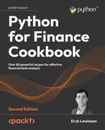
Which returns the following DataFrame containing intraday price data.
Figure 1.8: Preview of the downloaded intraday prices
Get Coca-Cola’s latest earnings record
Another interesting usage of the security_api is to recover the latest earnings records. We can do this using the following snippet:
r = security_api.get_security_latest_earnings_record(identifier="KO")
print(r)
The output of the API call contains quite a lot of useful information. For example, we can see what time of day the earnings call happened. This information could potentially be used for implementing trading strategies that act when the market opens.

Figure 1.9: Coca-Cola’s latest earnings record
See also
- https://docs.intrinio.com/documentation/api_v2/getting_started—the starting point for exploring the API
- https://docs.intrinio.com/documentation/api_v2/limits—an overview of the querying limits
- https://docs.intrinio.com/developer-sandbox—an overview of what is included in the free sandbox environment
- https://docs.intrinio.com/documentation/python—thorough documentation of the Python SDK
Getting data from Alpha Vantage
Alpha Vantage is another popular data vendor providing high-quality financial data. Using their API, we can download the following:
- Stock prices, including intraday and real-time (paid access)
- Fundamentals: earnings, income statement, cash flow, earnings calendar, IPO calendar
- Forex and cryptocurrency exchange rates
- Economic indicators such as real GDP, Federal Funds Rate, Consumer Price Index, and consumer sentiment
- 50+ technical indicators
In this recipe, we show how to download a selection of crypto-related data. We start with historical daily Bitcoin prices, and then show how to query the real-time crypto exchange rate.
Getting ready
Before downloading the data, we need to register at https://www.alphavantage.co/support/#api-key to obtain the API key. Access to the API and all the endpoints is free of charge (excluding the real-time stock prices) within some bounds (5 API requests per minute; 500 API requests per day).
How to do it…
Execute the following steps to download data from Alpha Vantage:
- Import the libraries:
from alpha_vantage.cryptocurrencies import CryptoCurrencies - Authenticate using your personal API key and select the API:
ALPHA_VANTAGE_API_KEY = "YOUR_KEY_HERE" crypto_api = CryptoCurrencies(key=ALPHA_VANTAGE_API_KEY, output_format= "pandas") - Download the daily prices of Bitcoin, expressed in EUR:
data, meta_data = crypto_api.get_digital_currency_daily(
    symbol="BTC",
    market="EUR"
)
The
meta_dataobject contains some useful information about the details of the query. You can see it below:{'1. Information': 'Daily Prices and Volumes for Digital Currency', '2. Digital Currency Code': 'BTC', '3. Digital Currency Name': 'Bitcoin', '4. Market Code': 'EUR', '5. Market Name': 'Euro', '6. Last Refreshed': '2022-08-25 00:00:00', '7. Time Zone': 'UTC'}The
dataDataFrame contains all the requested information. We obtained 1,000 daily OHLC prices, the volume, and the market capitalization. What is also noteworthy is that all the OHLC prices are provided in two currencies: EUR (as we requested) and USD (the default one).
Figure 1.10: Preview of the downloaded prices, volume, and market cap
- Download the real-time exchange rate:
crypto_api.get_digital_currency_exchange_rate(
    from_currency="BTC",
    to_currency="USD"
)[0].transpose()
Running the command returns the following DataFrame with the current exchange rate:

Figure 1.11: BTC-USD exchange rate
How it works…
After importing the alpha_vantage library, we had to authenticate using the personal API key. We did so while instantiating an object of the CryptoCurrencies class. At the same time, we specified that we would like to obtain output in the form of a pandas DataFrame. The other possibilities are JSON and CSV.
In Step 3, we downloaded the daily BTC prices using the get_digital_currency_daily method. Additionally, we specified that we wanted to get the prices in EUR. By default, the method will return the requested EUR prices, as well as their USD equivalents.
Lastly, we downloaded the real-time BTC/USD exchange rate using the get_digital_currency_exchange_rate method.
There’s more...
So far, we have used the alpha_vantage library as a middleman to download information from Alpha Vantage. However, the functionalities of the data vendor evolve faster than the third-party library and it might be interesting to learn an alternative way of accessing their API.
- Import the libraries:
import requests import pandas as pd from io import BytesIO - Download Bitcoin’s intraday data:
AV_API_URL = "https://www.alphavantage.co/query"
parameters = {
    "function": "CRYPTO_INTRADAY",
    "symbol": "ETH",
    "market": "USD",
    "interval": "30min",
    "outputsize": "full",
    "apikey": ALPHA_VANTAGE_API_KEY
}
r = requests.get(AV_API_URL, params=parameters)
data = r.json()
df = (
    pd.DataFrame(data["Time Series Crypto (30min)"])
    .transpose()
)
df
Running the snippet above returns the following preview of the downloaded DataFrame:

Figure 1.12: Preview of the DataFrame containing Bitcoin’s intraday prices
We first defined the base URL used for requesting information via Alpha Vantage’s API. Then, we defined a dictionary containing the additional parameters of the request, including the personal API key. In our function call, we specified that we want to download intraday ETH prices expressed in USD and sampled every 30 minutes. We also indicated we want a full output (by specifying the
outputsizeparameter). The other option iscompactoutput, which downloads the 100 most recent observations.Having prepared the request’s parameters, we used the
getfunction from therequestslibrary. We provide the base URL and theparametersdictionary as arguments. After obtaining the response to the request, we can access it in JSON format using thejsonmethod. Lastly, we convert the element of interest into apandasDataFrame.Alpha Vantage’s documentation shows a slightly different approach to downloading this data, that is, by creating a long URL with all the parameters specified there. Naturally, that is also a possibility, however, the option presented above is a bit neater. To see the very same request URL as presented by the documentation, you can run
r.request.url.
- Download the upcoming earnings announcements within the next three months:
AV_API_URL = "https://www.alphavantage.co/query"
parameters = {
    "function": "EARNINGS_CALENDAR",
    "horizon": "3month",
    "apikey": ALPHA_VANTAGE_API_KEY
}
r = requests.get(AV_API_URL, params=parameters)
pd.read_csv(BytesIO(r.content))

Figure 1.13: Preview of a DataFrame containing the downloaded earnings information
While getting the response to our API request is very similar to the previous example, handling the output is much different.
The output of r.content is a bytes object containing the output of the query as text. To mimic a normal file in-memory, we can use the BytesIO class from the io module. Then, we can normally load that mimicked file using the pd.read_csv function.
In the accompanying notebook, we present a few more functionalities of Alpha Vantage, such as getting the quarterly earnings data, downloading the calendar of the upcoming IPOs, and using alpha_vantage's TimeSeries module to download stock price data.
See also
- https://www.alphavantage.co/—Alpha Vantage homepage
- https://www.alphavantage.co/documentation/—the API documentation
- https://github.com/RomelTorres/alpha_vantage—the GitHub repo of the third-party library used for accessing data from Alpha Vantage
Getting data from CoinGecko
The last data source we will cover is dedicated purely to cryptocurrencies. CoinGecko is a popular data vendor and crypto-tracking website, on which you can find real-time exchange rates, historical data, information about exchanges, upcoming events, trading volumes, and much more.
We can list a few of the advantages of CoinGecko:
- Completely free, and no need to register for an API key
- Aside from prices, it also provides updates and news about crypto
- It covers many coins, not only the most popular ones
In this recipe, we download Bitcoin’s OHLC from the last 14 days.
How to do it…
Execute the following steps to download data from CoinGecko:
- Import the libraries:
from pycoingecko import CoinGeckoAPI from datetime import datetime import pandas as pd - Instantiate the CoinGecko API:
cg = CoinGeckoAPI() - Get Bitcoin’s OHLC prices from the last 14 days:
ohlc = cg.get_coin_ohlc_by_id(
    id="bitcoin", vs_currency="usd", days="14"
)
ohlc_df = pd.DataFrame(ohlc)
ohlc_df.columns = ["date", "open", "high", "low", "close"]
ohlc_df["date"] = pd.to_datetime(ohlc_df["date"], unit="ms")
ohlc_df

Figure 1.14: Preview of the DataFrame containing the requested Bitcoin prices
In the preceding table, we can see that we have obtained the requested 14 days of data, sampled every 4 hours.
How it works…
After importing the libraries, we instantiated the CoinGeckoAPI object. Then, using its get_coin_ohlc_by_id method we downloaded the last 14 days’ worth of BTC/USD exchange rates. It is worth mentioning there are some limitations of the API:
- We can only download data for a predefined number of days. We can select one of the following options:
1/7/14/30/90/180/365/max. - The OHLC candles are sampled with a varying frequency depending on the requested horizon. They are sampled every 30 minutes for requests of 1 or 2 days. Between 3 and 30 days they are sampled every 4 hours. Above 30 days, they are sampled every 4 days.
The output of the get_coin_ohlc_by_id is a list of lists, which we can convert into a pandas DataFrame. We had to manually create the column names, as they were not provided by the API.
There’s more...
We have seen that getting the OHLC prices can be a bit more difficult using the CoinGecko API as compared to the other vendors. However, CoinGecko has additional interesting information we can download using its API. In this section, we show a few possibilities.
Get the top 7 trending coins
We can use CoinGecko to acquire the top 7 trending coins—the ranking is based on the number of searches on CoinGecko within the last 24 hours. While downloading this information, we also get the coins’ symbols, their market capitalization ranking, and the latest price in BTC:
trending_coins = cg.get_search_trending()
(
    pd.DataFrame([coin["item"] for coin in trending_coins["coins"]])
    .drop(columns=["thumb", "small", "large"])
)
Using the snippet above, we obtain the following DataFrame:

Figure 1.15: Preview of the DataFrame containing the 7 trending coins and some information about them
Get Bitcoin’s current price in USD
We can also extract current crypto prices in various currencies:
cg.get_price(ids="bitcoin", vs_currencies="usd")
Running the snippet above returns Bitcoin’s real-time price:
{'bitcoin': {'usd': 47312}}
In the accompanying notebook, we present a few more functionalities of pycoingecko, such as getting the crypto price in different currencies than USD, downloading the entire list of coins supported on CoinGecko (over 9,000 coins), getting each coin’s detailed market data (market capitalization, 24h volume, the all-time high, and so on), and loading the list of the most popular exchanges.
See also
You can find the documentation of the pycoingecko library here: https://github.com/man-c/pycoingecko.
Summary
In this chapter, we have covered a few of the most popular sources of financial data. However, this is just the tip of the iceberg. Below, you can find a list of other interesting data sources that might suit your needs even better.
Additional data sources are:
- IEX Cloud (https://iexcloud.io/)—a platform providing a vast trove of different financial data. A notable feature that is unique to the platform is a daily and minutely sentiment score based on the activity on Stocktwits—an online community for investors and traders. However, that API is only available in the paid plan. You can access the IEX Cloud data using
pyex, the official Python library. - Tiingo (https://www.tiingo.com/) and the
tiingolibrary. - CryptoCompare (https://www.cryptocompare.com/)—the platform offers a wide range of crypto-related data via their API. What stands out about this data vendor is that they provide order book data.
- Twelve Data (https://twelvedata.com/).
- polygon.io (https://polygon.io/)—a trusted data vendor for real-time and historical data (stocks, forex, and crypto). Trusted by companies such as Google, Robinhood, and Revolut.
- Shrimpy (https://www.shrimpy.io/) and
shrimpy-python—the official Python library for the Shrimpy Developer API.
In the next chapter, we will learn how to preprocess the downloaded data for further analysis.
Join us on Discord!
To join the Discord community for this book – where you can share feedback, ask questions to the author, and learn about new releases – follow the QR code below: