- In the early 90s, neural networks had largely gone out of fashion. The bulk of machine learning research was around other techniques, such as random forests and support vector machines. Neural networks with only a single hidden layer were less performant than these other techniques, and it was thought that deeper neural networks were too difficult to train.
- The resurgence of interest in neural networks was spearheaded by Geoffrey Hinton, who, in 2004, led a team of researchers who proceeded to make a series of breakthroughs using restricted Boltzmann machines (RBM) and creating neural networks with many layers; they called this approach deep learning. Within 10 years, deep learning would go from being a niche technique to dominating every single AI competition. RBMs were part of the big breakthrough, allowing Hinton and others to get world record scores on a variety of image and speech recognition problems.
- In this section, we will look at the theory of how RBMs work, how to implement them, and how they can be combined into deep belief networks.
A restricted Boltzmann machine looks a lot like a single layer of a neural network. There are a set of input nodes that have connections to another set of output nodes:

Figure 1. Restricted Boltzmann machine
The way these output nodes are activated is also identical to an autoencoder. There is a weight between each input node and output node, the activation of each input nodes multiplied by this matrix of weight mappings, and a bias vector is then applied, and the sum for each output node is then put through a sigmoid function.
What makes a restricted Boltzmann machine different is what the activations represent, how we think about them, and the way in which they are trained. To begin with, when talking about RBMs rather than talking about input and output layers, we refer to the layers as visible and hidden. This is because, when training, the visible nodes represent the known information we have. The hidden nodes will aim to represent some variables that generated the visible data. This contrasts with an autoencoder, where the output layer doesn't explicitly represent anything, is just a constrained space through which the information is passed.
The basis of learning the weights of a restricted Boltzmann machine comes from statistical physics and uses an energy-based model (EBM). In these, every state is put through an energy function, which relates to the probability of a state occurring. If an energy function returns a high value, we expect this state to be unlikely, rarely occurring. Conversely, a low result from an energy function means a state that is more stable and will occur more frequently.
A good intuitive way of thinking about an energy function is to imagine a huge number of bouncy balls being thrown into a box. At first, all the balls have high energy and so will be bouncing very high. A state here would be a single snapshot in time of all the balls' positions and their associated velocities. These states, when the balls are bouncing, are going to be very transitory; they will only exist for moments and because of the range of movement of the balls, are very unlikely to reoccur. But as the balls start to settle, as the energy leaves the system, some of the balls will start to be increasingly stationary. These states are stable once it occurs once it never stops occurring. Eventually, once the balls have stopped bouncing and all become stationary, we have a completely stable state, which has high probability.
- To give an example that applies to restricted Boltzmann machines, consider the task of learning a group of images of butterflies. We train our RBM on these images, and we want it to assign a low energy value to any image of a butterflies. But when given an image from a different set, say cars, it will give it a high energy value. Related objects, such as moths, bats, or birds, may have a more medium energy value.
- If we have an energy function defined, the probability of a given state is then given as follows:

- Here, v is our state, E is our energy function, and Z is the partition function; the sum of all possible configurations of v is defined as follows:

- Before we go further into restricted Boltzmann machines, let's briefly talk about Hopfield networks; this should help in giving us a bit more of an understanding about how we get to restricted Boltzmann machines. Hopfield networks are also energy-based models, but unlike a restricted Boltzmann machine, it has only visible nodes, and they are all interconnected. The activation of each node will always be either -1 or +1.

Figure 2. Hopfield network, all input nodes are interconnected
- When running a Hopfield network (or RBM), you have two options. The first option is that you can set the value of every visible node to the corresponding value of your data item you are triggering it on. Then you can trigger successive activations, where, at each activation, every node has its value updated based on the value of the other visible nodes it is connected to. The other option is to just initialize the visible nodes randomly and then trigger successive activations so it produces random examples of the data it has been trained on. This is often referred to as the network daydreaming.
- The activation of each of these visible nodes at the next time step is defined as follows:

- Here, W is a matrix defining the connection strength between each node v at time step t. A thresholding rule is then applied to a to get a new state for v:

- The weights W between nodes can be either positive or negative, which will lead nodes to attract or repel the other nodes in the network, when active. The Hopfield network also has a continuous variant, which simply involves replacing the thresholding function with the tanh function.
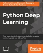
- The energy function for this network is as follows:

- In matrix notation, it is as follows:
- The
 in the equation is because we are going through every pair of i and j and so double-counting each connection (once when i=1 and j=2 then again when i=2 and j=1).
- The question that might arise here is: why have a model with only visible nodes? I will activate it with data I give it, then trigger some state updates. But what useful information does this new state give me? This is where the properties of energy-based models become interesting. Different configurations of W will vary the energy function associated with the states v. If we set the state of the network to something with a high energy function, that is an unstable state (think of the many bouncing balls); the network will over successive iterations move to a stable state.
- If we train a Hopefield network on a dataset to learn a W with low energy for each item in the dataset, we can then make a corrupted sample from the data, say, by randomly swapping a few of the inputs between their minus one and plus one states. The corrupted samples may be in a high-energy state now because the corruption has made it unlikely to be a member of the original dataset. If we activate the visible nodes of the network on the corrupted sample, run a few more iterations of the network until it has reached a low-energy state; there is a good chance that it will have reconstructed the original uncorrupted pattern.
- This leads to one use of the Hopfield networks being spelling correction; you can train it on a library of words, with the letters used in the words as inputs. Then if it is given a misspelled word, it may be able to find the correct original word. Another use of the Hopfield networks is as a content-addressable memory. One of the big differences between the computer memory and the human memory is that with computers, memories are stored with addresses. If a computer wants to retrieve a memory, it must know the exact place it stored it in. Human memory, on the other hand, can be given a partial section of that memory, the content of which can be used to recover the rest of it. For example, if I need to remember my pin number, I know the content I'm looking for and the properties of that content, a four digit number; my brain uses that to return the values.
- Hopfield networks allow you to store content-addressable memories, which have led some people to suggest (speculatively) that the human memory system may function like a Hopfield network, with human dreaming being the attempt to learn the weights.
- The last use of a Hopfield network is that it can be used to solve optimization tasks, such as the traveling salesman task. The energy function can be defined to represent the cost of the task to be optimized, and the nodes of the network to represent the choices being optimized. Again, all that needs to be done is to minimize the energy function with respect to the weights of the network.
- A Boltzmann machine is also known as a stochastic Hopfield network. In a Hopfield network, node activations are set based on the threshold; but in a Boltzmann machine, activation is stochastic. The value of a node in a Boltzmann machine is always set to either +1 or -1. The probability of the node being in the state +1 is defined as follows:

- Here, ai is the activation for that node as defined for the Hopfield network.
To learn the weights of our Boltzmann machine or Hopfield network, we want to maximize the likelihood of the dataset, given the W, which is simply the product of the likelihood for each data item:

Here, W is the weights matrix, and x(n) is the nth sample from the dataset x of size N. Let's now replace ![]() with the actual likelihood from our Boltzmann machine:
with the actual likelihood from our Boltzmann machine:

Here, Z is as shown in the following equation:

If you look at the original definition of our energy function and Z, then x' should be every possible configuration of x based on the probability distribution p(x). We now have W as part of our model, so the distribution will change to ![]() . Unfortunately,
. Unfortunately, ![]() is, if not completely intractable, at the very least, far too computationally expensive to compute. We would need to take every possible configuration of x across all possible W.
is, if not completely intractable, at the very least, far too computationally expensive to compute. We would need to take every possible configuration of x across all possible W.
One approach to computing an intractable probability distribution such as this is what's called Monte Carlo sampling. This involves taking lots of samples from the distribution and using the average of these samples to approximate the true value. The more samples we take from the distribution, the more accurate it will tend to be. A hypothetical infinite number of samples would be exactly the quantity we want, while 1 would be a very poor approximation.
Since the products of probabilities can get very small, we will instead use the log probability; also, let's also include the definition of Z:

Here, x' is a sample of state of the network, as taken from the probability distribution ![]() learned by the network. If we take the gradient of this with respect to a single weight between nodes i and j, it looks like this:
learned by the network. If we take the gradient of this with respect to a single weight between nodes i and j, it looks like this:

Here, ![]() across all N samples is simply the correlation between the nodes i and j. Another way to write this across all N samples, for each weight i and j, would be this:
across all N samples is simply the correlation between the nodes i and j. Another way to write this across all N samples, for each weight i and j, would be this:

This equation can be understood as being two phases of learning, known as positive and negative or, more poetically, waking and sleeping. In the positive phase, ![]() increases the weights based on the data we are given. In the negative phase,
increases the weights based on the data we are given. In the negative phase,  , we draw samples from the model as per the weights we currently have, then move the weights away from that distribution. This can be thought of as reducing the probability of items generated by the model. We want our model to reflect the data as closely as possible, so we want to reduce the selection generated by our model. If our model was producing images exactly like the data, then the two terms would cancel each other out, and equilibrium would be reached.
Boltzmann machines and Hopfield networks can be useful for tasks such as optimization and recommendation systems. They are very computationally expensive. Correlation must be measured between every single node, and then a range of Monte Carlo samples must be generated from the model for every training step. Also, the kinds of patterns it can learn are limited. If we are training on images to learn shapes, it cannot learn position invariant information. A butterfly on the left-hand side of an image is a completely different beast to a butterfly on the right-hand side of an image. In Chapter 5, Image Recognition, we will take a look at convolutional neural networks, which offers a solution to this problem.
Restricted Boltzmann machines make two changes from the Boltzmann machines: the first is that we add in hidden nodes, each of which is connected to every visible node, but not to each other. The second is that we remove all connections between visible nodes. This has the effect of making each node in the visible layer conditionally independent of each other if we are given the hidden layer. Nodes in the hidden layer are also conditionally independent, given the visible layer. We will also now add bias terms to both the visible and hidden nodes. A Boltzmann machine can also be trained with a bias term for each node, but this was left out of the equations for ease of notation.
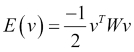
- Given that the data we have is only for the visible units, what we aim to do through training is find configurations of hidden units that lead to low-energy states when combined with the visible units. In our restricted Boltzmann machine, the state x is now the full configuration of both visible and hidden nodes. So, we will parameterize our energy function as E(v, h). It now looks like this:
- Here, a is the bias vector for the visible nodes, b is the bias vector for the hidden nodes, and W is the matrix of weights between the visible and hidden nodes. Here,
 is the dot product of the two vectors, equivalent to
  . Now we need to take the gradients of our biases and weights with respect to this new energy function.
- Because of the conditional independence between layers, we now have this:
-
These two definitions will be used in the normalization constant, Z. Since we longer have connections between visible nodes, our
 has changed a lot:

- Here, i is going through each visible node and j through each hidden node. If we take the gradient with respect to the different parameters, then what you eventually end up with is this:


As before, ![]() is approximated by taking the Monte Carlo samples from the distribution. These final three equations give us the complete way to iteratively train all the parameters for a given dataset. Training will be a case of updating our parameters by some learning rate by these gradients.
is approximated by taking the Monte Carlo samples from the distribution. These final three equations give us the complete way to iteratively train all the parameters for a given dataset. Training will be a case of updating our parameters by some learning rate by these gradients.
It is worth restating on a conceptual level what is going on here. v denotes the visible variables, the data from the world on which we are learning. h denotes the hidden variables, the variables we will train to generate visible variables. The hidden variables do not explicitly represent anything, but through training and minimizing the energy in the system, they should eventually find important components of the distribution we are looking at. For example, if the visible variables are a list of movies, with a value of 1 if a person likes the movie and 0 if they do not, the hidden variables may come to represent genres of movie, such as horror or comedy, because people may have genre preferences, so this is an efficient way to encode people's tastes.
If we generate random samples of hidden variables and then activate the visible variables based on this, it should give us a plausible looking set of human tastes in movies. Likewise, if we set the visible variables to a random selection of movies over successive activations of the hidden and visible nodes, it should move us to find a more plausible selection.
Now that we have gone through the math, let's see what an implementation of it looks like. For this, we will use TensorFlow. TensorFlow is a Google open source mathematical graph library that is popular for deep learning. It does not have built-in neural network concepts, such as network layers and nodes, which a higher-level library such as Keres does; it is closer to a library such as Theano. It has been chosen here because being able to work directly on the mathematical symbols underlying the network allows the user to get a better understanding of what they are doing.
TensorFlow can be installed directly via pip using the command pip install tensorflow for the CPU version or pip install tensorflow-gpu if you have NVidea GPU-enabled machine.
We will build a small restricted Boltzmann machine and train it on the MNIST collection of handwritten digits. We will have a smaller number of hidden nodes than visible nodes, which will force the RBM to learn patterns in the input. The success of the training will be measured in the network's ability to reconstruct the image after putting it through the hidden layer; for this, we will use the mean squared error between the original and our reconstruction. The full code sample is in the GitHub repo https://github.com/DanielSlater/PythonDeepLearningSamples in the restricted_boltzmann_machine.py file.
Since the MNIST dataset is used so ubiquitously, TensorFlow has a nice built-in way to download and cache the MNIST dataset. It can be done by simply calling the following code:
from tensorflow.examples.tutorials.mnist import input_data
mnist = input_data.read_data_sets("MNIST_data/")
This will download all the MNIST data into MNIST_data into the "MNIST_data/" directory, if it is not already there. The mnist object has properties, train and test, which allow you to access the data in NumPy arrays. The MNIST images are all sized 28 by 28, which means 784 pixels per image. We will need one visible node in our RBM for each pixel:
input_placeholder = tf.placeholder("float", shape=(None, 784))A placeholder object in TensorFlow represents values that will be passed in to the computational graph during usage. In this case, the input_placeholder object will hold the values of the MNIST images we give it. The "float" specifies the type of value we will be passing in, and the
shape defines the dimensions. In this case, we want 784 values, one for each pixel, and the None dimension is for batching. Having a None dimension means that it can be of any size; so, this will allow us to send variable-sized batches of 784-length arrays:
weights = tf.Variable(tf.random_normal((784, 300), mean=0.0, stddev=1./784))
tf.variable represents a variable on the computational graph. This is the W from our preceding equations. The argument passed to it is how the variable values should first be initialized. Here, we are initializing it from a normal distribution of size 784 by 300, the number of visible nodes to hidden nodes:
hidden_bias = tf.Variable(tf.zeros([300]))
visible_bias = tf.Variable(tf.zeros([784]))
These variables will be the a and b from our preceding equation; they are initialised to all start with a value of 0. Now we will program in the activations of our network:
hidden_activation = tf.nn.sigmoid(tf.matmul(input_placeholder, weights) + hidden_bias)
This represents the activation of the hidden nodes, ![]() , in the preceding equations. After applying the
, in the preceding equations. After applying the sigmoid function, this activation could be put into a binomial distribution so that all values in the hidden layer go to 0 or 1, with the probability given; but it turns out an RBM trains just as well as the raw probabilities. So, there's no need to complicate the model by doing this:
visible_reconstruction = tf.nn.sigmoid(tf.matmul(hidden_activation, tf.transpose(weights)) + visible_bias)
Now we have the reconstruction of the visible layer, ![]() . As specified by the equation, we give it the
. As specified by the equation, we give it the hidden_activation, and from that, we get our sample from the visible layer:
final_hidden_activation = tf.nn.sigmoid(tf.matmul(visible_reconstruction, weights) + hidden_bias)
We now compute the final sample we need, the activation of the hidden nodes from our visible_reconstruction. This is equivalent to ![]() in the equations. We could keep going with successive iterations of hidden and visual activation to get a much more unbiased sample from the model. But it doing just one rotation works fine for training:
in the equations. We could keep going with successive iterations of hidden and visual activation to get a much more unbiased sample from the model. But it doing just one rotation works fine for training:
Positive_phase = tf.matmul(tf.transpose(input_placeholder), hidden_activation)
Negative_phase = tf.matmul(tf.transpose(visible_reconstruction), final_hidden_activation)
Now we compute the positive and negative phases. The first phase is the correlation across samples from our mini-batch of the input_placeholder,
![]() and the first
and the first hidden_activation, ![]() . Then the negative phase gets the correlation between the
. Then the negative phase gets the correlation between the visible_reconstruction, ![]() and the
and the final_hidden_activation, ![]() :
:
LEARING_RATE = 0.01
weight_update = weights.assign_add(LEARING_RATE * (positive_phase – negative_phase))
Calling assign_add on our weights variable creates an operation that, when run, adds the given quantity to the variable. Here, 0.01 is our learning rate, and we scale the positive and negative phases by that:
visible_bias_update = visible_bias.assign_add(LEARING_RATE * tf.reduce_mean(input_placeholder - visible_reconstruction, 0))
hidden_bias_update = hidden_bias.assign_add(LEARING_RATE * tf.reduce_mean(hidden_activation - final_hidden_activation, 0))
Now we create the operations for scaling the hidden and visible biases. These are also scaled by our 0.01 learning rate:
train_op = tf.group(weight_update, visible_bias_update, hidden_bias_update)Calling tf.group creates a new operation than when called executes all the operation arguments together. We will always want to update all the weights in unison, so it makes sense to create a single operation for them:
loss_op = tf.reduce_sum(tf.square(input_placeholder - visible_reconstruction))This loss_op will give us feedback on how well we are training, using the MSE. Note that this is purely used for information; there is no backpropagation run against this signal. If we wanted to run this network as a pure autoencoder, we would create an optimizer here and activate it to minimize the loss_op:?
session = tf.Session()
session.run(tf.initialize_all_variables())
Then we create a session object that will be used for running the computational graph. Calling tf.initialize_all_variables() is when everything gets initialized on to the graph. If you are running TensorFlow on the GPU, this is where the hardware is first interfaced with. Now that we have created every step for the RBM, let's put it through a few epochs of running against MNIST and see how well it learns:
current_epochs = 0

for i in range(10):
    total_loss = 0
    while mnist.train.epochs_completed == current_epochs:
        batch_inputs, batch_labels = mnist.train.next_batch(100)
        _, reconstruction_loss = session.run([train_op, loss_op], feed_dict={input_placeholder: batch_inputs})
        total_loss += reconstruction_loss

    print("epochs %s loss %s" % (current_epochs, reconstruction_loss))
    current_epochs = mnist.train.epochs_completed
Every time we call mnist.train.next_batch(100), 100 images are retrieved from the mnist dataset. At the end of each epoch, the mnist.train.epochs_completed is incremented by 1, and all the training data is reshuffled. If you run this, you may see results something like this:
epochs 0 loss 1554.51
epochs 1 loss 792.673
epochs 2 loss 572.276
epochs 3 loss 479.739
epochs 4 loss 466.529
epochs 5 loss 415.357
epochs 6 loss 424.25
epochs 7 loss 406.821
epochs 8 loss 354.861
epochs 9 loss 410.387
epochs 10 loss 313.583
We can now see what an image reconstruction looks like by running the following command on the mnist data:
reconstruction = session.run(visible_reconstruction, feed_dict={input_placeholder:[mnist.train.images[0]]})Here are some examples of what the reconstructed images with 300 hidden nodes look like:

Figure 3. Reconstructions of digits using restricted Boltzmann machines with different numbers of hidden nodes
As you can see, with 300 hidden nodes, less than half the number of pixels, it can still do an almost perfect reconstruction of the image, with only a little blurring around the edges. But as the number of hidden nodes decreases, so does the quality of the reconstruction. Going down to just 10 hidden nodes, the reconstructions can produce images that, to the human eye, look like the wrong digit, such as the 2 and 3 in Figure 3.
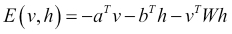
If we imagine our RBM is learning a set of latent variables that generated our visible data and we were feeling inquisitive, we might wonder: can we then learn a second layer of latent variables that generated the latent variables for the hidden layer? The answer is yes, we can stack RBMs on top of previously trained RBMs to be able to learn second, third, fourth, and so on, order information about the visible data. These successive layers of RBMs allow the network to learn increasingly invariant representations of the underlying structure:
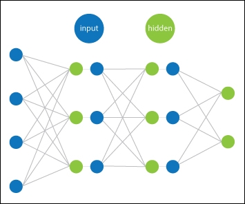
Figure 4 Deep belief network, containing many chained RBMs
These stacked RBMs are known as deep belief networks and were the deep networks used by Geoffrey Hinton in his 2002 paper Training Products of Experts by Minimizing Contrastive Divergence, to first produce the record-breaking results on MNIST. The exact technique he found useful was to train successive RBMs on data with only a slight reduction in the size of the layers. Once a layer was trained to the point where the reconstruction error was no longer improving, its weights were frozen, and a new RBM was stacked on top and again trained until error rate convergence. Once the full network was trained, a final supervised layer was put at the end in order to map the final RBM's hidden layer to the labels of the data. Then the weights of the whole network were used to construct a standard deep feed-forward neutral network, allowing those precalculated weights of the deep belief network to be updated by backpropagation.
At first, these had great results, but over time, the techniques for training standard feed-forward networks have improved, and RBMs are no longer considered the best for image or speech recognition. They also have the problem that because of their two-phase nature, they can be a lot slower to train. But they are still very popular for things such as recommender systems and pure unsupervised learning. Also, from a theoretical point of view, using the energy-based model to learn deep representations is a very interesting approach and leaves the door open for many extensions that can be built on top of this approach.