One of the reasons why deep neural networks can succeed where other traditional machine learning techniques struggle is the capability of learning the right representations of entities in the data (features) without needing (much) human and domain knowledge.
Theoretically, neural networks are able to consume raw data directly as it is and map the input layers to the desired output via the hidden intermediate representations. Traditional machine learning techniques focus mainly on the final mapping and assume the task of "feature engineering" to have already been done.
Feature engineering is the process that uses the available domain knowledge to create smart representations of the data, so that it can be processed by the machine learning algorithm.
Andrew Yan-Tak Ng is a professor at Stanford University and one of the most renowned researchers in the field of machine learning and artificial intelligence. In his publications and talks, he describes the limitations of traditional machine learning when applied to solving real-world problems.
The hardest part of making a machine learning system work is to find the right feature representations:
Coming up with features is difficult, time-consuming, requires expert knowledge. When working applications of learning, we spend a lot of time tuning features.
Anrew Ng, Machine Learning and AI via Brain simulations, Stanford University
Let's assume we are classifying pictures into a few categories, such as animals versus vehicles. The raw data is a matrix of the pixels in the image. If we used those pixels directly in a logistic regression or a decision tree, we would create rules (or associating weights) for every single picture that might work for the given training samples, but that would be very hard to generalize enough to small variations of the same pictures. In other words, let's suppose that my decision tree finds that there are five important pixels whose brightness (supposing we are displaying only black and white tones) can determine where most of the training data get grouped into the two classes--animals and vehicles. The same pictures, if cropped, shifted, rotated, or re-colored, would not follow the same rules as before. Thus, the model would probably randomly classify them. The main reason is that the features we are considering are too weak and unstable. However, we could instead first preprocess the data such that we could extract features like these:
- Does the picture contain symmetric centric, shapes like wheels?
- Does it contain handlebars or a steering wheel?
- Does it contain legs or heads?
- Does it have a face with two eyes?
In such cases, the decision rules would be quite easy and robust, as follows:
How much effort is needed in order to extract those relevant features?
Since we don't have handlebar detectors, we could try to hand-design features to capture some statistical properties of the picture, for example, finding edges in different orientations in different picture quadrants. We need to find a better way to represent images than pixels.
Moreover, robust and significant features are generally made out of hierarchies of previously extracted features. We could start extracting edges in the first step, then take the generated "edges vector", and combine them to recognize object parts, such as an eye, a nose, a mouth, rather than a light, a mirror, or a spoiler. The resulting object parts can again be combined into object models; for example, two eyes, one nose, and one mouth form a face, or two wheels, a seat, and a handlebar form a motorcycle. The whole detection algorithm could be simplified in the following way:
By recursively applying sparse features, we manage to get higher-level features. This is why you need deeper neural network architectures as opposed to the shallow algorithms. The single network can learn how to move from one representation to the following, but stacking them together will enable the whole end-to-end workflow.
The real power is not just in the hierarchical structures though. It is important to note that we have only used unlabeled data so far. We are learning the hidden structures by reverse-engineering the data itself instead of relying on manually labeled samples. The supervised learning represents only the final classification steps, where we need to assign to either the vehicle class or the animal class. All of the previous steps are performed in an unsupervised fashion.
We will see how the specific feature extraction for pictures is done in the following Chapter 5, Image Recognition. In this chapter, we will focus on the general approach of learning feature representations for any type of data (for example, time signals, text, or general attribute vectors).
For that purpose, we will cover two of the most powerful and quite used architectures for unsupervised feature learning: autoencoders and restricted Boltzmann machines.
Autoencoders are symmetric networks used for unsupervised learning, where output units are connected back to input units:

Autoencoder simple representation from H2O training book (https://github.com/h2oai/h2o-training-book/blob/master/hands-on_training/images/autoencoder.png)
The output layer has the same size of the input layer because its purpose is to reconstruct its own inputs rather than predicting a dependent target value.
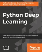
The goal of those networks is to act as a compression filter via an encoding layer, Φ that fits the input vector X into a smaller latent representation (the code) c, and then a decoding layer, Φ tries to reconstruct it back to X':
The loss function is the reconstruction error, which will force the network to find the most efficient compact representation of the training data with minimum information loss. For numerical input, the loss function can be the mean squared error:
If the input data is not numerical but is represented as a vector of bits or multinomial distributions, we can use the cross-entropy of the reconstruction:

Here, d is the dimensionality of the input vectors.
The central layer (the code) of the network is the compressed representation of the data. We are effectively translating an n-dimensional array into a smaller m-dimensional array, where m < n. This process is very similar to dimensionality reduction using Principal Component Analysis (PCA). PCA divides the input matrix into orthogonal axes (called components) in such, way that you can reconstruct an approximation of the original matrix by projecting the original points on those axes. By sorting them by their importance, we can extract the top m components that can be though as high-level features of the original data.
For example, in a multivariate Gaussian distribution, we could represent each point as a coordinate over the two orthogonal components that would describe the largest possible variance in the data:

A scatter plot of samples that are distributed according a multivariate (bivariate) Gaussian distribution centered at (1,3) with a standard deviation of 3 in the (0.866, 0.5) direction and of 1 in the orthogonal direction. The directions represent the principal components (PC) associated with the sample. By Nicoguaro (own work) CC BY 4.0 (http://creativecommons.org/licenses/by/4.0), via Wikimedia Commons.
The limitation of PCA is that it allows only linear transformation of the data, which is not always enough.
Autoencoders have the advantage of being able to represent even non-linear representations using a non-linear activation function.
One famous example of an autoencoder was given by MITCHELL, T. M. in his book Machine Learning, wcb, 1997. In that example, we have a dataset with eight categorical objects encoded in binary with eight mutually exclusive labels with bits. The network will learn a compact representation with just three hidden nodes:

Tom Mitchell's example of an autoencoder.
By applying the right activation function, the learn-compact representation corresponds exactly with the binary representation with three bits.
There are situations though where just the single hidden layer is not enough to represent the whole complexity and variance of the data. Deeper architecture can learn more complicated relationships between the input and hidden layers. The network is then able to learn latent features and use those to best represent the non-trivial informative components in the data.
A deep autoencoder is obtained by concatenating two symmetrical networks typically made of up to five shallow layers:

Schematic structure of an autoencoder with 3 fully-connected hidden layers (https://en.wikipedia.org/wiki/Autoencoder#/media/File:Autoencoder_structure.png)
Deep autoencoders can learn new latent representations, combining the previously learned ones so that each hidden level can be seen as some compressed hierarchical representation of the original data. We could then use the code or any other hidden layer of the encoding network as valid features describing the input vector.
Probably the most common question when building a deep neural network is: how do we choose the number of hidden layers and the number of neurons for each layer? Furthermore, which activation and loss functions do we use?
There is no closed answer. The empirical approach consists of running a sequence of trial and error or a standard grid search, where the depth and the size of each layer are simply defined as tuning hyperparameters. We will look at a few design guidelines.
For autoencoders, the problem is slightly simplified. Since there are many variants of autoencoders, we will define the guidelines for the general use case. Please keep in mind that each variation will have its own rules to be considered. We can suggest the following:
- The output layer consists of exactly the same size of the input.
- The network is symmetric most of the time. Having an asymmetric network would mean having different complexities of the encoder and decoder functions. Unless you have a particular reason for doing so, there is generally no advantage in having asymmetric networks. However, you could decide to share the same weights or decide to have different weights in the encoding and decoding networks.
- During the encoding phase, the hidden layers are smaller than the input, in which case, we are talking about "undercomplete autoencoders". A multilayer encoder gradually decreases the representation size. The size of the hidden layer, generally, is at most half the size of the previous one. If the data input layer has 100 nodes, then a plausible architecture could be 100-40-20-40-100. Having bigger layers than the input would lead to no compression at all, which means no interesting patterns are learned. We will see in the Regularization section how this constraint is not necessary in case of sparse autoencoders.
- The middle layer (the code) covers an important role. In the case of feature reduction, we could keep it small and equal to 2, 3, or 4 in order to allow efficient data visualizations. In the case of stacked autoencoders, we should set it to be larger because it will represent the input layer of the next encoder.
- In the case of binary inputs, we want to use sigmoid as the output activation function and cross-entropy, or more precisely, the sum of Bernoulli cross-entropies, as the loss function.
- For real values, we can use a linear activation function (ReLU or softmax) as the output and the mean squared error (MSE) as the loss function.
- For different types of input data(x)and output u, you can follow the general approach, which consists of the following steps:
- Finding the probability distribution of observing x, given u, P(x/u)
- Finding the relationship between u and the hidden layer h(x)
- Using
- In the case of deep networks (with more than one hidden layer), use the same activation function for all of them in order to not unbalance the complexity of the encoder and decoder.
- If we use a linear activation function throughout the whole network, we will approximate the behavior of PCA.
- It is convenient to Gaussian scale (0 mean and unit standard deviation) your data unless it is binary, and it is better to leave the input values to be either 0 or 1. Categorical data can be represented using one-hot-encoding with dummy variables.
- Activation functions are as follows:
- ReLU is generally the default choice for majority of neural networks. Autoencoders, given their topology, may benefit from a symmetric activation function. Since ReLU tends to overfit more, it is preferred when combined with regularization techniques (such as dropout).
- If your data is binary or can be scaled in the range of [0, 1], then you would probably use a sigmoid activation function. If you used one-hot-encoding for the input categorical data, then it's better use ReLU.
- Hyperbolic tangent (tanh) is a good choice for computation optimization in case of gradient descent. Since data will be centered around 0, the derivatives will be higher. Another effect is reducing bias in the gradients as is well explained in the "Efficient BackProp" paper (http://yann.lecun.com/exdb/publis/pdf/lecun-98b.pdf).

Different activation functions commonly used for deep neural networks
In the previous chapters, we already saw different forms of regularizations, such as L1, L2, early stopping, and dropout. In this section, we will describe a few popular techniques specifically tailored for autoencoders.
So far, we have always described autoencoders as "undercomplete", which means the hidden layers are smaller than the input layer. This is because having a bigger layer would have no compression at all. The hidden units may just copy exactly the input and return an exact copy as the output.
On the other hand, having more hidden units would allow us to have more freedom on learning smarter representations.
We will see how we can address this problem with three approaches: denoising autoencoders, contractive autoencoders, and sparse autoencoders.
The idea is that we want to train our model to learn how to reconstruct a noisy version of the input data.
We will use x to represent the original input, ![]() , the noisy input, and
, the noisy input, and ![]() , the reconstructed output.
, the reconstructed output.
The noisy input, ![]() , is generated by randomly assigning a subset of the input
, is generated by randomly assigning a subset of the input ![]() to 0, with a given probability ?, plus an additive isotropic Gaussian noise, with variance v for numerical inputs.
to 0, with a given probability ?, plus an additive isotropic Gaussian noise, with variance v for numerical inputs.
We would then have two new hyper-parameters to tune ?? and ![]() , which represent the noise level.
, which represent the noise level.
We will use the noisy variant, ![]() , as the input of the network, but the loss function will still be the error between the output
, as the input of the network, but the loss function will still be the error between the output ![]() and the original noiseless input
and the original noiseless input ![]() . If the input dimensionality is d, the encoding function f, and the decoding function g, we will write the loss function j as this:
. If the input dimensionality is d, the encoding function f, and the decoding function g, we will write the loss function j as this:

Here, L is the reconstruction error, typically either the MSE or the cross-entropy.
With this variant, if a hidden unit tries to exactly copy the input values, then the output layer cannot trust 100% because it knows that it could be the noise and not the original input. We are forcing the model to reconstruct based on the interrelationships between other input units, aka the meaningful structures of the data.
What we would expect is that the higher the added noise, the bigger the filters applied at each hidden unit. By filter, we mean the portion of the original input that is activated for that particular feature to be extracted. In case of no noise, hidden units tend to extract a tiny subset of the input data and propose it at the most untouched version to the next layer. By adding noise to the units, the error penalty on badly reconstructing ![]() will force the network to keep more information in order to contextualize the features regardless of the possible presence of noise.
will force the network to keep more information in order to contextualize the features regardless of the possible presence of noise.
Please pay attention that just adding a small white noise could be equivalent to using weight decay regularization. Weight decay is a technique that consists of multiplying to a factor less than 1 the weights at each training epoch in order to limit the free parameters in our model. Although this is a popular technique to regularize neural networks, by setting inputs to 0 with probability p, we are effectively achieving a totally different result.
We don't want to obtain high-frequency filters that when put together give us a more generalized model. Our denoising approach generates filters that do represent unique features of the underlying data structures and have individual meanings.
Contractive autoencoders aim to achieve a similar goal to that of the denoising approach by explicitly adding a term that penalizes when the model tries to learn uninteresting variations and promote only those variations that are observed in the training set.
In other words, the model may try to approximate the identity function by coming out with filters representing variations that are not necessarily present in the training data.
We can express this sensitivity as the sum of squares of all partial derivatives of the extracted features with respect to the input dimensions.
For an input x of dimensionality ![]() mapped by the encoding function f to the hidden representation h of size dh, the following quantity corresponds to the L2 norm (Frobenius) of the Jacobian matrix
mapped by the encoding function f to the hidden representation h of size dh, the following quantity corresponds to the L2 norm (Frobenius) of the Jacobian matrix ![]() of the encoder activations:
of the encoder activations:

The loss function will be modified as follows:
Here, λ is the regularization factor. It is easy to see that the Frobenius norm of the Jacobian corresponds to L2 weight decay in the case of a linear encoder. The main difference is that for the linear case, the only way of achieving contraction would be by keeping weights very small. In case of a sigmoid non-linearity, we could also push the hidden units to their saturated regime.
Let's analyze the two terms.
The error J (the MSE or cross-entropy) pushes toward keeping the most possible information to perfectly reconstruct the original value.
The penalty pushes toward getting rid of all of that information such that the derivatives of the hidden units with respect to X are minimized. A large value means that the learned representation is too unstable with respect to input variations. We obtain a small value when we observe very little change to the hidden representations as we change the input values. In case of the limit of these derivatives being 0, we would only keep the information that is invariant with respect to the input X. We are effectively getting rid of all of the hidden features that are not stable enough and too sensitive to small perturbations.
Let's suppose we have as input a lot of variations of the same data. In the case of images, they could be small rotations or different exposures of the same subject. In case of network traffic, they could be an increase/decrease of the packet header of the same type of traffic, maybe because of a packing/unpacking protocol.
If we only look at this dimension, the model is likely to be very sensitive. The Jacobian term would penalize the high sensitivity, but it is compensated by the low reconstruction error.
In this scenario, we would have one unit that is very sensitive on the variation direction but not very useful for all other directions. For example, in the case of pictures, we still have the same subject; thus, all of the remaining input values are constant. If we don't observe variations on a given direction in the training data, we want to discard the feature.
H2O currently does not support contractive autoencoders; however, an open issue can be found at https://0xdata.atlassian.net/browse/PUBDEV-1265.
Autoencoders, as we have seen them so far, always have the hidden layers smaller than the input.
The major reason is that otherwise, the network would have enough capability to just memorize exactly the input and reconstruct it perfectly as it is. Adding extra capacity to the network would just be redundant.
Reducing the capacity of the network forces to learn based on a compression version of the input. The algorithm will have to pick the most relevant features that help better reconstruct the training data.
There are situations though where compressing is not feasible. Let's consider the case where each input node is formed by independent random variables. If the variables are not correlated with each other, the only way of achieving compression is to get rid of some of them entirely. We are effectively emulating the behavior of PCA.
In order to solve this problem, we can set a sparsity constraint on the hidden units. We will try to push each neuron to be inactive most of the time that corresponds to having the output of the activation function close to 0 for sigmoid and ReLU, -1 for tanh.
If we call ![]() the activation of hidden unit
the activation of hidden unit ![]() at layer
at layer ![]() when input is
when input is ![]() , we can define the average activation of hidden unit
, we can define the average activation of hidden unit ![]() as follows:
as follows:

Here, ![]() is the size of our training dataset (or batch of training data).
is the size of our training dataset (or batch of training data).
The sparsity constraint consists of forcing ![]() , where
, where ![]() is the sparsity parameter bounded in the interval [1,0] and ideally close enough to 0.
is the sparsity parameter bounded in the interval [1,0] and ideally close enough to 0.
The original paper (http://web.stanford.edu/class/cs294a/sparseAutoencoder.pdf) recommends values near 0.05.
We model the average activation of each hidden unit as a Bernoulli random variable with mean ![]() , and we want to force all of them to converge to a Bernoulli distribution with mean
, and we want to force all of them to converge to a Bernoulli distribution with mean ![]()
In order to do so, we need to add an extra penalty that quantifies the divergence of those two distributions. We can define this penalty based on the Kullback-Leibler (KL) divergence between the real distribution ![]() and the theoretical one
and the theoretical one ![]() we would like to achieve.
we would like to achieve.
In general, for discrete probability distributions P and Q, the KL divergence when information is measured in bits is defined as follows:

One requirement is that P is absolutely continuous with respect to Q, that is, ![]() for any measurable value of x. This is also written as
for any measurable value of x. This is also written as ![]() . Whenever
. Whenever ![]() , the contribution of that term will be
, the contribution of that term will be ![]() since that
since that ![]() .
.
In our case, the ![]() divergence of unit j would be as follows:
divergence of unit j would be as follows:

This function has the property to be ![]() when the two means are equal and increase monotonically, otherwise until approaching 8 when
when the two means are equal and increase monotonically, otherwise until approaching 8 when ![]() is close to
is close to
or 1.
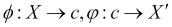
The final loss function with extra penalty term added will be this:
Here, J is the standard loss function (the RMSE), ![]() is the number of hidden units, and ß is a weight of the sparsity term.
is the number of hidden units, and ß is a weight of the sparsity term.
This extra penalty will cause a small inefficiency to the backpropagation algorithm. In particular, the preceding formula will require an additional forward step over the whole training set to precompute the average activations ![]() before computing the backpropagation on each example.
before computing the backpropagation on each example.
Autoencoders are powerful unsupervised learning algorithms, which are getting popularity in fields such as anomaly detection or feature engineering, using the output of intermediate layers as features to train a supervised model instead of the raw input data.
Unsupervised means they do not require labels or ground truth to be specified during training. They just work with whatever data you put as input as long as the network has enough capability to learn and represent the intrinsic existing relationships. That means that we can set both the size of the code layer (the reduced dimensionality m) but obtain different results depending on the number and size of the hidden layers, if any.
If we are building an autoencoder network, we want to achieve robustness in order to avoid wrong representations but at the same time not limit the capacity of the network by compressing the information through smaller sequential layers.
Denoising, contractive, and autoencoders are all great techniques for solving those problems.
Adding noise is generally simpler and doesn't add complexity in the loss function, which results in less computation. On the other hand, the noisy input makes the gradient to be sampled and also discard part of the information in exchange for better features.
Contractive autoencoders are very good at making the model more stable to small deviations from the training distribution. Thus, it is a very good candidate for reducing false alarms. The drawback is a sort of countereffect that increases the reconstruction error in order to reduce the sensibility.
Sparse autoencoders are probably the most complete around solution. It is the most expensive to compute for large datasets, but since the gradient is deterministic, it can be useful in case of second-order optimizers and, in general, to provide a good trade-off between stability and low reconstruction error.
Regardless of what choice you make, adopting a regularization technique is strongly recommended. They both come with hyper-parameters to tune, which we will see how to optimize in the corresponding Tuning section.
In addition to the techniques described so far, it is worth mentioning variational autoencoders, which seem to be the ultimate solution for regularizing autoencoders. Variational autoencoders belong to the class of generative models. They don't just learn the structures that better describe the training data, they learn the parameters of a latent unit Gaussian distribution that can best regenerate the input data. The final loss function will be the sum of the reconstruction error and the KL divergence between the reconstructed latent variable and the Gaussian distribution. The encoder phase will generate a code consisting of a vector of means and a vector of standard deviations. From the code, we can characterize the latent distribution parameters and reconstruct the original input by sampling from that distribution.