Chapter 2
Storing Data in Hadoop
WHAT’S IN THIS CHAPTER?
- Getting to know the Hadoop Distributed File System (HDFS)
- Understanding HBase
- Choosing the most appropriate data storage for your applications
WROX.COM CODE DOWNLOADS FOR THIS CHAPTER
The wrox.com code downloads for this chapter are found at http://www.wiley.com/go/prohadoopsolutions on the Download Code tab. The code is in the Chapter 2 download and individually named according to the names throughout the chapter.
The foundation of efficient data processing in Hadoop is its data storage model. This chapter examines different options for storing data in Hadoop — specifically, in the Hadoop Distributed File System (HDFS) and HBase. This chapter explores the benefits and drawbacks of each option, and outlines a decision tree for picking the best option for a given problem. You also learn about Apache Avro — an Hadoop framework for data serialization, which can be tightly integrated with Hadoop-based storage. This chapter also covers different data access models that can be implemented on top of Hadoop storage.
HDFS
HDFS is Hadoop’s implementation of a distributed filesystem. It is designed to hold a large amount of data, and provide access to this data to many clients distributed across a network. To be able to successfully leverage HDFS, you first must understand how it is implemented and how it works.
HDFS Architecture
The HDFS design is based on the design of the Google File System (GFS). Its implementation addresses a number of problems that are present in a number of distributed filesystems such as Network File System (NFS). Specifically, the implementation of HDFS addresses the following:
- To be able to store a very large amount of data (terabytes or petabytes), HDFS is designed to spread the data across a large number of machines, and to support much larger file sizes compared to distributed filesystems such as NFS.
- To store data reliably, and to cope with the malfunctioning or loss of individual machines in the cluster, HDFS uses data replication.
- To better integrate with Hadoop’s MapReduce, HDFS allows data to be read and processed locally. (Data locality is discussed in more detail in Chapter 4.)
The scalability and high-performance design of HDFS comes with a price. HDFS is restricted to a particular class of applications — it is not a general-purpose distributed filesystem. A large number of additional decisions and trade-offs govern HDFS architecture and implementation, including the following:
- HDFS is optimized to support high-streaming read performance, and this comes at the expense of random seek performance. This means that if an application is reading from HDFS, it should avoid (or at least minimize) the number of seeks. Sequential reads are the preferred way to access HDFS files.
- HDFS supports only a limited set of operations on files — writes, deletes, appends, and reads, but not updates. It assumes that the data will be written to the HDFS once, and then read multiple times.
- HDFS does not provide a mechanism for local caching of data. The overhead of caching is large enough that data should simply be re-read from the source, which is not a problem for applications that are mostly doing sequential reads of large-sized data files.
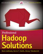
HDFS is implemented as a block-structured filesystem. As shown in Figure 2-1, individual files are broken into blocks of a fixed size, which are stored across an Hadoop cluster. A file can be made up of several blocks, which are stored on different DataNodes (individual machines in the cluster) chosen randomly on a block-by-block basis. As a result, access to a file usually requires access to multiple DataNodes, which means that HDFS supports file sizes far larger than a single-machine disk capacity.
FIGURE 2-1: HDFS architecture
The DataNode stores each HDFS data block in a separate file on its local filesystem with no knowledge about the HDFS files themselves. To improve throughput even further, the DataNode does not create all files in the same directory. Instead, it uses heuristics to determine the optimal number of files per directory, and creates subdirectories appropriately.
One of the requirements for such a block-structured filesystem is the capability to store, manage, and access file metadata (information about files and blocks) reliably, and to provide fast access to the metadata store. Unlike HDFS files themselves (which are accessed in a write-once and read-many model), the metadata structures can be modified by a large number of clients concurrently. It is important that this information never gets out of sync. HDFS solves this problem by introducing a dedicated special machine, called the NameNode, which stores all the metadata for the filesystem across the cluster. This means that HDFS implements a master/slave architecture. A single NameNode (which is a master server) manages the filesystem namespace and regulates access to files by clients. The existence of a single master in a cluster greatly simplifies the architecture of the system. The NameNode serves as a single arbitrator and repository for all HDFS metadata.
Because of the relatively low amount of metadata per file (it only tracks filenames, permissions, and the locations of each block), the NameNode stores all of the metadata in the main memory, thus allowing for a fast random access. The metadata storage is designed to be compact. As a result, a NameNode with 4 GB of RAM is capable of supporting a huge number of files and directories.
Metadata storage is also persistent. The entire filesystem namespace (including the mapping of blocks to files and filesystem properties) is contained in a file called the FsImage stored as a file in the NameNode’s local filesystem. The NameNode also uses a transaction log to persistently record every change that occurs in filesystem metadata (metadata store). This log is stored in the EditLog file on the NameNode’s local filesystem.
To keep the memory footprint of the NameNode manageable, the default size of an HDFS block is 64 MB — orders of magnitude larger than the block size of the majority of most other block-structured filesystems. The additional benefit of the large data block is that it allows HDFS to keep large amounts of data stored on the disk sequentially, which supports fast streaming reads of data.
The downside of HDFS file organization is that several DataNodes are involved in the serving of a file, which means that a file can become unavailable in the case where any one of those machines is lost. To avoid this problem, HDFS replicates each block across a number of machines (three, by default).
Data replication in HDFS is implemented as part of a write operation in the form of a data pipeline. When a client is writing data to an HDFS file, this data is first written to a local file. When the local file accumulates a full block of data, the client consults the NameNode to get a list of DataNodes that are assigned to host replicas of that block. The client then writes the data block from its local storage to the first DataNode (see Figure 2-1) in 4K portions. The DataNode stores the received blocks in a local filesystem, and forwards that portion of data to the next DataNode in the list. The same operation is repeated by the next receiving DataNode until the last node in the replica set receives data. This DataNode stores data locally without sending it any further.
If one of the DataNodes fails while the block is being written, it is removed from the pipeline. In this case, when the write operation on the current block completes, the NameNode re-replicates it to make up for the missing replica caused by the failed DataNode. When a file is closed, the remaining data in the temporary local file is pipelined to the DataNodes. The client then informs the NameNode that the file is closed. At this point, the NameNode commits the file creation operation into a persistent store. If the NameNode dies before the file is closed, the file is lost.
The default block size and replication factor are specified by Hadoop configuration, but can be overwritten on a per-file basis. An application can specify block size, the number of replicas, and the replication factor for a specific file at its creation time.
One of the most powerful features of HDFS is optimization of replica placement, which is crucial to HDFS reliability and performance. All decisions regarding replication of blocks are made by the NameNode, which periodically (every 3 seconds) receives a heartbeat and a block report from each of the DataNodes. A heartbeat is used to ensure proper functioning of DataNodes, and a block report allows verifying that a list of blocks on a DataNode corresponds to the NameNode information. One of the first things that a DataNode does on startup is sending a block report to the NameNode. This allows the NameNode to rapidly form a picture of the block distribution across the cluster.
An important characteristic of the data replication in HDFS is rack awareness. Large HDFS instances run on a cluster of computers that is commonly spread across many racks. Typically, network bandwidth (and consequently network performance) between machines in the same rack is greater than network bandwidth between machines in different racks.
The NameNode determines the rack ID that each DataNode belongs to via the Hadoop Rack Awareness process. A simple policy is to place replicas on unique racks. This policy prevents losing data when an entire rack is lost, and evenly distributes replicas in the cluster. It also allows using bandwidth from multiple racks when reading data. But because a write must, in this case, transfer blocks to multiple racks, the performance of writes suffers.
An optimization of a Rack Aware policy is to cut inter-rack write traffic (and consequently improve write performance) by using the number of racks that is less than the number of replicas. For example, when a replication factor is three, two replicas are placed on one rack, and the third one is on a different rack.
To minimize global bandwidth consumption and read latency, HDFS tries to satisfy a read request from a replica that is closest to the reader. If a replica exists on the same rack as the reader node, that replica is used to satisfy the read request.
As mentioned, each DataNode periodically sends a heartbeat message to the NameNode (see Figure 2-1), which is used by the NameNode to discover DataNode failures (based on missing heartbeats). The NameNode marks DataNodes without recent heartbeats as dead, and does not dispatch any new I/O requests to them. Because data located at a dead DataNode is no longer available to HDFS, DataNode death may cause the replication factor of some blocks to fall below their specified values. The NameNode constantly tracks which blocks must be re-replicated, and initiates replication whenever necessary.
HDFS supports a traditional hierarchical file organization similar to most other existing filesystems. It supports creation and removal of files within a directory, moving files between directories, and so on. It also supports user’s quota and read/write permissions.
Using HDFS Files
Now that you know how HDFS works, this section looks at how to work with HDFS files. User applications access the HDFS filesystem using an HDFS client, a library that exposes the HDFS filesystem interface that hides most of the complexities of HDFS implementation described earlier. The user application does not need to know that filesystem metadata and storage are on different servers, or that blocks have multiple replicas.
Access to HDFS is through an instance of the FileSystem object. A FileSystem class is an abstract base class for a generic filesystem. (In addition to HDFS, Apache provides implementation of FileSystem objects for other filesystems, including KosmosFileSystem, NativeS3FileSystem, RawLocalFileSystem, and S3FileSystem.) It may be implemented as a distributed filesystem, or as a “local” one that uses the locally connected disk. The local version exists for small Hadoop instances and for testing. All user code that may potentially use HDFS should be written to use a FileSystem object.
You can create an instance of the FileSystem object by passing a new Configuration object into a constructor. Assuming that Hadoop configuration files (hadoop-default.xml and hadoop-site.xml) are available on the class path, the code snippet shown in Listing 2-1 creates an instance of FileSystem object. (Configuration files are always available if the execution is done on one of the Hadoop cluster’s nodes. If execution is done on the remote machine, the configuration file must be explicitly added to the application class path.)
LISTING 2-1: Creating a FileSystem object
Configuration conf = new Configuration();
FileSystem fs = FileSystem.get(conf);
Another important HDFS object is Path, which represents names of files or directories in a filesystem. A Path object can be created from a string representing the location of the file/directory on the HDFS. A combination of FileSystem and Path objects allows for many programmatic operations on HDFS files and directories. Listing 2-2 shows an example.
LISTING 2-2: Manipulating HDFS objects
Path filePath = new Path(file name);
......................................................
if(fs.exists(filePath))
     //do something
......................................................
if(fs.isFile(filePath))
     //do something
......................................................
Boolean result = fs.createNewFile(filePath);
......................................................
Boolean result = fs.delete(filePath);
......................................................
FSDataInputStream in = fs.open(filePath);
FSDataOutputStream out = fs.create(filePath);
The last two lines in Listing 2-2 show how to create FSDataInputStream and FSDataOutputStream objects based on a file path. These two objects are subclasses of DataInputStream and DataOutputStream from the Java I/O package, which means that they support standard I/O operations.
With this in place, an application can read/write data to/from HDFS the same way data is read/written from the local data system.
Hadoop-Specific File Types
In addition to “ordinary” files, HDFS also introduced several specialized files types (such as SequenceFile, MapFile, SetFile, ArrayFile, and BloomMapFile) that provide much richer functionality, which often simplifies data processing.
SequenceFile provides a persistent data structure for binary key/value pairs. Here, different instances of both key and value must represent the same Java class, but can have different sizes. Similar to other Hadoop files, SequenceFiles are append-only.
When using an ordinary file (either text or binary) for storing key/value pairs (typical data structures for MapReduce), data storage is not aware of key and value layout, which must be implemented in the readers on top of generic storage. The use of SequenceFile provides a storage mechanism natively supporting key/value structure, thus making implementations using this data layout much simpler.
SequenceFile has three available formats: Uncompressed, Record-Compressed, and Block-Compressed. The first two are stored in a record-based format (shown in Figure 2-2), whereas the third one uses block-based format (shown in Figure 2-3).
FIGURE 2-2: Record-based SequenceFile format

FIGURE 2-3: Block-based SequenceFile format

The choice of a specific format for a sequence file defines the length of the file on the hard drive. Block-Compressed files typically are the smallest, while Uncompressed are the largest.
In Figure 2-2 and Figure 2-3, the header contains general information about SequenceFiles, as shown in Table 2-1.
TABLE 2-1: SequenceFile Header
| FIELD | DESCRIPTION |
| Version | A 4-byte array containing three letters (SEQ) and a sequence file version number (either 4 or 6). The currently used version is 6. Version 4 is supported for backward compatibility. |
| Key Class | Name of the key class, which is validated against a name of the key class provided by the reader. |
| Value class | Name of the value class, which is validated against a name of the key class provided by the reader. |
| Compression | A key/value compression flag. |
| Block Compression | A block compression flag. |
| Compression Codec | CompressionCodec class. This class is used only if either key/value or block compression flag are true. Otherwise, this value is ignored. |
| Metadata | A metadata (optional) is a list of key/value pairs, which can be used to add user-specific information to the file. |
| Sync | A sync marker. |
As shown in Table 2-2, a record contains the actual data for keys and values, along with their lengths.
TABLE 2-2: Record Layout
| FIELD | DESCRIPTION |
| Record length | The length of the record (bytes) |
| Key Length | The length of the key (bytes) |
| Key | Byte array, containing the record’s key |
| Value | Byte array, containing the record’s value |
In this case, header and sync are serving the same purpose as in the case of a record-based SequenceFile format. The actual data is contained in the blocks, as shown in Table 2-3.
TABLE 2-3: Block Layout
| FIELD | DESCRIPTION |
| Keys lengths length | In this case, all the keys for a given block are stored together. This field specifies compressed key-lengths size (in bytes) |
| Keys Lengths | Byte array, containing compressed key-lengths block |
| Keys length | Compressed keys size (in bytes) |
| Keys | Byte array, containing compressed keys for a block |
| Values lengths length | In this case, all the values for a given block are stored together. This field specifies compressed value-lengths block size (in bytes) |
| Values Lengths | Byte array, containing compressed value-lengths block |
| Values length | Compressed values size (in bytes) |
| Values | Byte array, containing compressed values for a block |
All formats use the same header that contains information allowing the reader to recognize it. The header (see Table 2-1) contains key and value class names that are used by the reader to instantiate those classes, the version number, and compression information. If compression is enabled, the Compression Codec class name field is added to the header.
Metadata for the SequenceFile is a set of key/value text pairs that can contain additional information about the SequenceFile that can be used by the file reader/writer.
Implementation of write operations for Uncompressed and Record-Compressed formats is very similar. Each call to an append() method adds a record containing the length of the whole record (key length plus value length), the length of the key, and the raw data of key and value to the SequenceFile. The difference between the compressed and the uncompressed version is whether or not the raw data is compressed, with the specified codec.
The Block-Compressed format applies a more aggressive compression. Data is not written until it reaches a threshold (block size), at which point all keys are compressed together. The same thing happens for the values and the lists of key and value lengths.
A special reader (SequenceFile.Reader) and writer (SequenceFile.Writer) are provided by Hadoop for use with SequenceFiles. Listing 2-3 shows a small snippet of code using SequenceFile.Writer.
LISTING 2-3: Using SequenceFile.Writer
Configuration conf = new Configuration();
FileSystem fs = FileSystem.get(conf);
Path path = new Path("fileName");
SequenceFile.Writer sequenceWriter = new SequenceFile.Writer(fs, conf, path,
           Key.class,value.class,fs.getConf().getInt("io.file.buffer.size",
4096),fs.getDefaultReplication(), 1073741824, null,new Metadata());

.......................................................................
sequenceWriter.append(bytesWritable, bytesWritable);
..........................................................
IOUtils.closeStream(sequenceWriter);
A minimal SequenceFile writer constructor (SequenceFile.Writer(FileSystem fs, Configuration conf, Path name, Class keyClass, Class valClass)) requires the specification of the filesystem, Hadoop configuration, path (file location), and definition of both key and value classes. A constructor that is used in the previous example enables you to specify additional file parameters, including the following:
- int bufferSize — The default buffer size (4096) is used, if it is not defined.
- short replication — Default replication is used.
- long blockSize — The value of 1073741824 (1024 MB) is used.
- Progressable progress — None is used.
- SequenceFile.Metadata metadata — An empty metadata class is used.
Once the writer is created, it can be used to add key/record pairs to the file.
One of the limitations of SequenceFile is the inability to seek based on the key values. Additional Hadoop file types (MapFile, SetFile, ArrayFile, and BloomMapFile) enable you to overcome this limitation by adding a key-based index on top of SequenceFile.
As shown in Figure 2-4, a MapFile is really not a file, but rather a directory containing two files — the data (sequence) file, containing all keys and values in the map, and a smaller index file, containing a fraction of the keys. You create MapFiles by adding entries in order. MapFiles are typically used to enable an efficient search and retrieval of the contents of the file by searching on their index.
FIGURE 2-4: MapFile

The index file is populated with the key and a LongWritable that contains the starting byte position of the record corresponding to this key. An index file does not contain all the keys, but just a fraction of them. You can set the indexInterval using setIndexInterval() method on the writer. The index is read entirely into memory, so for the large map, it is necessary to set an index skip value that allows making the index file small enough so that it fits in memory completely.
Similar to the SequenceFile, a special reader (MapFile.Reader) and writer (MapFile.Writer) are provided by Hadoop for use with map files.
SetFile and ArrayFile are variations of MapFile for specialized implementations of key/value types. The SetFile is a MapFile for the data represented as a set of keys with no values (a value is represented by NullWritable instance). The ArrayFile deals with key/value pairs where keys are just a sequential long. It keeps an internal counter, which is incremented as part of every append call. The value of this counter is used as a key.
Both file types are useful for storing keys, not values.
Finally, the BloomMapFile extends the MapFile implementation by adding a dynamic bloom filter (see the sidebar, “Bloom Filters”) that provides a fast membership test for keys. It also offers a fast version of a key search operation, especially in the case of sparsely populated MapFiles. A writer’s append() operation updates a DynamicBloomFilter, which is then serialized when the writer is closed. This filter is loaded in memory when a reader is created. A reader’s get() operation first checks the filter for the key membership, and if the key is absent, it immediately returns null without doing any further I/O.
HDFS Federation and High Availability
The main limitation of the current HDFS implementation is a single NameNode. Because all of the file metadata is stored in memory, the amount of memory in the NameNodes defines the number of files that can be available on an Hadoop cluster. To overcome the limitation of a single NameNode memory and being able to scale the name service horizontally, Hadoop 0.23 introduced HDFS Federation, which is based on multiple independent NameNodes/namespaces.
Following are the main benefits of HDFS Federation:
- Namespace scalability — HDFS cluster storage scales horizontally, but the namespace does not. Large deployments (or deployments using a lot of small files) benefit from scaling the namespace by adding more NameNodes to the cluster.
- Performance — Filesystem operation throughput is limited by a single NameNode. Adding more NameNodes to the cluster scales the filesystem read/write operation’s throughput.
- Isolation — A single NameNode offers no isolation in a multi-user environment. An experimental application can overload the NameNode and slow down production-critical applications. With multiple NameNodes, different categories of applications and users can be isolated to different namespaces.
As shown in Figure 2-5, implementation of HDFS Federation is based on the collection of independent NameNodes that don’t require coordination with each other. The DataNodes are used as common storage for blocks by all the NameNodes. Each DataNode registers with all the NameNodes in the cluster. DataNodes send periodic heartbeats and block reports, and handle commands from the NameNodes.
FIGURE 2-5: HDFS Federation NameNode architecture

A namespace operates on a set of blocks — a block pool. Although a pool is dedicated to a specific namespace, the actual data can be allocated on any of the DataNodes in the cluster. Each block pool is managed independently, which allows a namespace to generate block IDs for new blocks without the need for coordination with the other namespaces. The failure of a NameNode does not prevent the DataNode from serving other NameNodes in the cluster.
A namespace and its block pool together are called a namespace volume. This is a self-contained unit of management. When a NameNode/namespace is deleted, the corresponding block pool at the DataNodes is deleted. Each namespace volume is upgraded as a unit, during cluster upgrade.
HDFS Federation configuration is backward-compatible, and allows existing single NameNode configuration to work without any change. The new configuration is designed such that all the nodes in the cluster have the same configuration without the need for deploying a different configuration based on the type of the node in the cluster.
Although HDFS Federation solves the problem of HDFS scalability, it does not solve the NameNode reliability issue. (In reality, it makes it worse — a probability of one NameNode failure in this case is higher.) Figure 2-6 shows a new HDFS high-availability architecture that contains two separate machines configured as NameNodes with exactly one of them in an active state at any point in time. The active NameNode is responsible for all client operations in the cluster, while the other one (standby) is simply acting as a slave, maintaining enough state to provide a fast failover if necessary. To keep state of both nodes synchronized, the implementation requires that both nodes have access to a directory on a shared storage device.
FIGURE 2-6: HDFS failover architecture

When any namespace modification is performed by the active node, it durably logs a record of the modification to a log file located in the shared directory. The standby node is constantly watching this directory for changes, and applies them to its own namespace. In the event of a failover, the standby ensures that it has read all of the changes before transitioning to the active state.
To provide a fast failover, it is also necessary for the standby node to have up-to-date information regarding the location of blocks in the cluster. This is achieved by configuring DataNodes to send block location information and heartbeats to both DataNodes.
Currently, only manual failover is supported. This limitation is eliminated by patches to core Hadoop committed to trunk and branch 1.1 by Hortonworks. This solution is based on a Hortonworks failover controller, which automatically picks an active NameNode.
HDFS provides very powerful and flexible support for storing large amounts of data. Special file types like SequenceFiles are very well suited for supporting MapReduce implementation. MapFiles and their derivatives (Set, Array, and BloomMap) work well for fast data access.
Still, HDFS supports only a limited set of access patterns — write, delete, and append. Although, technically, updates can be implemented as overwrites, the granularity of such an approach (overwrite will work only on the file level) can be cost-prohibitive in most cases. Additionally, HDFS design is geared toward supporting large sequential reads, which means that random access to the data can cause significant performance overhead. And, finally, HDFS is not well suited for a smaller file size. Although, technically, those files are supported by HDFS, their usage creates significant overhead in NameNode memory requirements, thus negatively impacting the upper limit of Hadoop’s cluster memory capacity.
To overcome many of these limitations, a more flexible data storage and access model was introduced in the form of HBase.
HBASE
HBase is a distributed, versioned, column-oriented, multidimensional storage system, designed for high performance and high availability. To be able to successfully leverage HBase, you first must understand how it is implemented and how it works.
HBase Architecture
HBase is an open source implementation of Google’s BigTable architecture. Similar to traditional relational database management systems (RDBMSs), data in HBase is organized in tables. Unlike RDBMSs, however, HBase supports a very loose schema definition, and does not provide any joins, query language, or SQL.
The main focus of HBase is on Create, Read, Update, and Delete (CRUD) operations on wide sparse tables. Currently, HBase does not support transactions (but provides limited locking support and some atomic operations) and secondary indexing (several community projects are trying to implement this functionality, but they are not part of the core HBase implementation). As a result, most HBase-based implementations are using highly denormalized data.
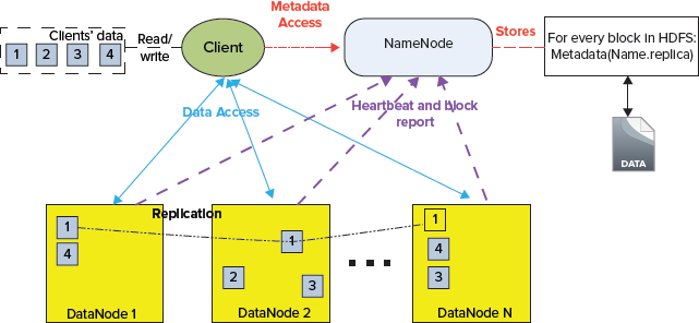
Similar to HDFS, HBase implements master/slave (HMaster/region server) architecture, as shown in Figure 2-7.
FIGURE 2-7: High-level HBase architecture
HBase leverages HDFS for its persistent data storage. This allows HBase to leverage all advanced features that HDFS provides, including checksums, replication, and failover. HBase data management is implemented by distributed region servers, which are managed by HBase master (HMaster).
A region server’s implementation consists of the following major components:
- memstore is HBase’s implementation of in-memory data cache, which allows improving the overall performance of HBase by serving as much data as possible directly from memory. The memstore holds in-memory modifications to the store in the form of key/values. A write-ahead-log (WAL) records all changes to the data. This is important in case something happens to the primary storage. If the server crashes, it can effectively replay that log to get everything up to where the server should have been just before the crash. It also means that if writing the record to the WAL fails, the whole operation must be considered a failure.
- HFile is a specialized HDFS file format for HBase. The implementation of HFile in a region server is responsible for reading and writing HFiles to and from HDFS.
A distributed HBase instance depends on a running Zookeeper cluster. (See the sidebar, “Zookeeper,” for a description of this service.) All participating nodes and clients must be able to access the running Zookeeper instances. By default, HBase manages a Zookeeper “cluster” — it starts and stops the Zookeeper processes as part of the HBase start/stop process. Because the HBase master may be relocated, clients bootstrap by looking to Zookeeper for the current location of the HBase master and -Root- table.
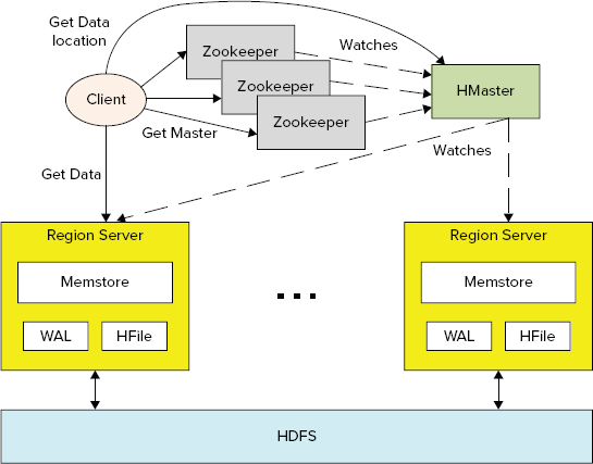
As shown in Figure 2-8, HBase uses an auto-sharding and distribution approach to cope with a large data size (compared to HDFS block-based design and fast data access).
FIGURE 2-8: Table sharding and distribution
To store a table of arbitrary length, HBase partitions this table into regions, with every region containing a sorted (by primary key), continuous range of rows. The term “continuous” here does not mean that a region contains all the keys from the given interval. Rather, it means that all keys from an interval are guaranteed to be partitioned to the same region, which can have any number of holes in a key space.
The way regions are split depends not on the key space, but rather on the data size. The size of data partition for a given table can be configured during table creation. These regions are “randomly” spread across region servers. (A single region server can serve any number of regions for a given table.) They can also be moved around for load balancing and failover.
When a new record is inserted in the table, HBase decides which region server it should go to (based on the key value) and inserts it there. If the region’s size exceeds the predefined one, the region automatically splits. The region split is a fairly expensive operation. To avoid some of it, the table can also be pre-split during creation, or manually at any point (more on this later in this chapter).
When a record (or set of records) is read/updated, HBase decides which regions should contain the data, and directs the client to the appropriate ones. From this point, region servers implement the actual read/update operation.
As shown in Figure 2-9, HBase leverages a specialized table (.META.) to resolve a specific key/table pair to the specific region server. This table contains a list of available region servers, and a list of descriptors for user tables. Each descriptor specifies a key range for a given table, contained in a given region.
FIGURE 2-9: Region server resolution in HBase

A .META. table is discovered using another specialized HBase table (-ROOT-), which contains a list of descriptors for a .META. table. A location of the –ROOT- table is held in Zookeeper.
As shown in Figure 2-10, an HBase table is a sparse, distributed, persistent multidimensional sorted map. The first map level is a key/row value. As mentioned, row keys are always sorted, which is the foundation of a table’s sharding and efficient reads and scans — reading of the key/value pairs in sequence.
FIGURE 2-10: Rows, column families, and columns
The second map level used by HBase is based on a column family. (Column families were originally introduced by columnar databases for fast analytical queries. In this case, data is stored not row by row as in a traditional RDBMS, but rather by column families.) Column families are used by HBase for separation of data based on access patterns (and size).
Column families play a special role in HBase implementation. They define how HBase data is stored and accessed. Every column family is stored in a separate HFILE. This is an important consideration to keep in mind during table design. It is recommended that you create a column family per data access type — that is, data typically read/written together should be placed in the same column family.
A set of the column families is defined during table creation (although it can be altered at a later point). Different column families can also use a different compression mechanism, which might be an important factor, for example, when separate column families are created for metadata and data (a common design pattern). In this case, metadata is often relatively small, and does not require compression, whereas data can be sufficiently large, and compression often allows improving HBase throughput.
Because of such a storage organization, HBase implements merged reads. For a given row, it reads all of the files of the column families and combines them together before sending them back to the client. As a result, if the whole row is always processed together, a single column family will typically provide the best performance.
The last map level is based on columns. HBase treats columns as a dynamic map of key/value pairs. This means that columns are not defined during table creation, but are dynamically populated during write/update operations. As a result, every row/column family in the HBase table can contain an arbitrary set of columns. The columns contain the actual values.
Technically, there is one more map level supported by HBase — versioning of every column value. HBase does not distinguish between writes and updates — an update is effectively a write with a new version. By default, HBase stores the last three versions for a given column value (while automatically deleting older versions). The depth of versioning can be controlled during table creation. A default implementation of the version is the timestamp of the data insertion, but it can be easily overwritten by a custom version value.
Following are the four primary data operations supported by HBase:
- Get returns values of column families/columns/versions for a specified row (or rows). It can be further narrowed to apply to a specific column family/column/version. It is important to realize that if Get is narrowed to a single column family, HBase would not have to implement a merged read.
- Put either adds a new row (or rows) to a table if the key does not exist, or updates an existing row (or rows) if the key already exists. Similar to Get, Put can be limited to apply to a specific column family/column.
- Scan allows iteration over multiple rows (a key range) for specified values, which can include the whole row, or any of its subset.
- Delete removes a row (or rows), or any part thereof from a table. HBase does not modify data in place, and, as a result, Deletes are handled by creating new markers called tombstones. These tombstones, along with the dead values, are cleaned up on major compactions. (You learn more about compactions later in this chapter.)
Get and Scan operations on HBase can be optionally configured with filters (filters are described later in this chapter), which are applied on the region server. They provide an HBase read optimization technique, enabling you to improve the performance of Get/Scan operations. Filters are effectively conditions that are applied to the read data on the region server, and only the rows (or parts of the rows) that pass filtering are delivered back to the client.
HBase supports a wide range of filters from row key to column family, and columns to value filters. Additionally, filters can be combined in the chains using boolean operations. Keep in mind that filtering does not reduce the amount of data read (and still often requires a full table scan), but can significantly reduce network traffic. Filter implementations must be deployed on the server, and require its restart.
In addition to general-purpose Put/Get operations, HBase supports the following specialized operations:
- Atomic conditional operations (including atomic compare and set) allow executing a server-side update, guarded by a check and atomic compare and delete (executing a server-side guarded Delete).
- Atomic “counters” increment operations, which guarantee synchronized operations on them. Synchronization, in this case, is done within a region server, not on the client.
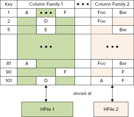
This is the logical view of HBase data. Table 2-4 describes the format that HBase uses to store the table data.
TABLE 2-4: Table Data Layout in the File

This table explains the mechanics used by HBase to deal with sparsely populated tables and arbitrary column names. HBase explicitly stores each column, defined for a specific key in an appropriate column family file.
Because HBase uses HDFS as a persistence mechanism, it never overwrites data. (HDFS does not support updates.) As a result, every time memstore is flushed to disk, it does not overwrite an existing store file, but rather creates a new one. To avoid proliferation of the store files, HBase implements a process known as compaction.
Two types of compaction exist: minor and major. Minor compactions usually pick up a couple of the smaller adjacent store files and rewrite them as one. Minor compactions do not drop Deletes or expired cells; only major compactions do this. Sometimes a minor compaction picks up all the store files, in which case it actually promotes itself to being a major compaction.
After a major compaction runs, there will be a single store file per store, which usually improves performance. Compactions will not perform region merges.
For faster key search within the files, HBase leverages bloom filters, which enable you to check on row or row/column level, and potentially filter an entire stored file from read. This filtering is especially useful in the case of a population of sparse keys. Bloom filters are generated when a file is persisted, and are stored at the end of each file.
HBase Schema Design
When designing an HBase schema, you should take the following general guidelines into consideration:
- The most effective access to HBase data is usage of Get or Scan operations based on the row key. HBase does not support any secondary keys/indexes. This means that, ideally, a row key should be designed to accommodate all of the access patterns required for a specific table. This often means using the composite row key to accommodate more data access patterns. (Best practices for row key design are discussed later in this chapter.)
- A general guideline is to limit the number of column families per table not to exceed 10 to 15. (Remember that every column family is stored by HBase in a separate file, so a large amount of column families are required to read and merge multiple files.) Also, based on the fact that the column family name is stored explicitly with every column name (see Table 2-4), you should minimize the size of the column family. Single-letter names are often recommended, if the amount of data in the column is small.
- Although HBase does not impose any limitation on the size of columns in a given row, you should consider the following:
- Rows are not splittable. As a result, a huge column data size (close to the region size) typically manifests that this type of data should not be stored in HBase.
- Each column value is stored along with its metadata (row key, column family name, column name), which means that a very small column data size leads to a very inefficient use of storage (that is, more space is occupied with metadata than the actual table data). It also implies that you should not use long column names.
- When deciding between tall-narrow (millions of keys with a limited amount of columns) versus flat-wide (a limited number of keys with millions of columns) table design, the former is generally recommended. This is because of the following:
- In the extreme cases, a flat-wide table might end up with one row per region, which is bad for performance and scalability.
- Table scans are typically more efficient compared to massive reads. As a result, assuming that only a subset of the row data is needed, a tall-narrow design provides better overall performance.
One of the main strengths of HBase design is the distributed execution of requests between multiple region servers. However, taking advantage of this design and ensuring that there are no “hot” (overloaded) servers during an application’s execution might require special design approaches for the row key. A general recommendation is to avoid a monotonically increasing sequence (for example, 1, 2, 3, or timestamps) as the row key for massive Put operations. You can mitigate any congestion in a single region brought on by monotonically increasing keys by randomizing the key values so that they are not in sorted order.
Data locality is also an important design consideration for HBase Get/Scan operations. Rows that are often retrieved together should be co-located, which means that they must have adjacent keys.
A general rule is to use sequential keys in the Scan-heavy cases, especially if you can leverage bulk imports for data population. Random keys are recommended for massive parallel writes with random, single key access.
The following are some specific row key design patterns:
- Key “salting” — This entails prefixing a sequential key with a random value, which allows for “bucketing” sequential keys across multiple regions.
- The swap/promotion of key fields (for example “reverse domains”) — A common design pattern in web analytics is to use a domain name as a row key. Using a reverse domain name as a key helps in this case by keeping information about pages per site close to each other.
- Complete randomization of keys — An example of this would be to use an MD5 hash.
A final consideration for the key design is the key size. Based on the information shown in Table 2-4, a key value is stored with every column value, which means that a key size should be sufficient for the effective search, but not any longer. Excessive key sizes will have negative impacts on the size of HBase store files.
Programming for HBase
HBase provides native Java, REST, and Thrift APIs. In addition, HBase supports a command-line interface and web access via HBase master web pages, both of which are well described in other HBase books, and are not tackled here. Because this book is aimed at the developers who access HBase from their applications, only the Java interface (which can be split into two major parts — data manipulation and administration) is discussed here.
All programmatic data-manipulation access to HBase is done through either the HTableInterface or the HTable class that implements HTableInterface. Both support all of the HBase major operations described previously, including Get, Scan, Put, and Delete.
Listing 2-4 shows how an instance of the HTable class can be created based on the table name.
LISTING 2-4: Creating an HTable instance
Configuration configuration = new Configuration();
HTable table = new HTable(configuration, "Table");
One thing to keep in mind is that HTable implementation is single-threaded. If it is necessary to have access to HBase from multiple threads, every thread must create its own instance of the HTable class. One of the ways to solve this problem is to use the HTablePool class. This class serves one purpose — pooling client API (HTableInterface) instances in the HBase cluster. Listing 2-5 shows an example of creating and using HTablePool.
LISTING 2-5: Creating and using an HTablePool instance
Configuration configuration = new Configuration();
HTablePool _tPool = new HTablePool(config, mSize);
....................................................................................
HTableInterface table = _tPool.getTable("Table");
....................................................................................
_tPool.putTable(table);
....................................................................................
_tPool.closeTablePool("testtable");
Once an appropriate class or an interface is obtained, all of the HBase operations, described previously (including Get, Scan, Put, and Delete), are available as its methods.
The small example in Listing 2-6 shows an implementation of the Get operation on the table "table" for key "key".
LISTING 2-6: Implementing a Get operation
HTable table = new HTable(configuration, "table");
Get get = new Get(Bytes.toBytes("key"));
Result result = table.get(get);
NavigableMap<byte[], byte[]> familyValues =  result.getFamilyMap(Bytes.toBytes
     "columnFamily"));
for(Map.Entry<byte[], byte[]> entry : familyValues.entrySet()){
     String column = Bytes.toString(entry.getKey);
     Byte[] value = entry.getValue();
     ...................................................................................................
}
Here, after getting the whole raw, only content of the column family "columnFamily" is required. This content is returned by HBase in the form of a navigable map, which can be iterated to get the values of the individual columns with their names.
Put and Delete are implemented by leveraging the same pattern. HBase also provides an important optimization technique in the form of a multi Get/Put, as shown in Listing 2-7.
LISTING 2-7: Implementing a multi-Put operation
Map<String, byte[]> rows = ...................;
HTable table = new HTable(configuration, "table");
List<Put> puts = new ArrayList<Put>();
for(Map.Entry<String, byte[]> row : rows.entrySet()){
     byte[] bkey = Bytes.toBytes(row.getKey());
     Put put = new Put(bkey);
put.add(Bytes.toBytes("family"), Bytes.toBytes("column"),row.getValue());
     puts.add(put);
}
table.put(puts);
...................................................................................................
In this code snippet, it is assumed that input comes in the form of a map containing a key and value, which should be written to a family called "family", column named "column". Instead of sending individual Put requests, a list of Put operations is created, and is sent as a single request. The actual performance improvements from usage of a multi Get/Put can vary significantly, but in general, this approach always seems to lead to better performance.
One of the most powerful operations provided by HBase is Scan, which allows iterating over a set of consecutive keys. Scan enables you to specify a multiplicity of parameters, including a start and end key, a set of column families and columns that will be retrieved, and a filter that will be applied to the data. Listing 2-8 (code file: class BoundinBoxFilterExample) shows an example of how to use Scan.
LISTING 2-8: Implementing a Scan operation
Put put = new Put(Bytes.toBytes("b"));
put.add(famA, coll1, Bytes.toBytes("0.,0."));
put.add(famA, coll2, Bytes.toBytes("hello world!"));
hTable.put(put);
put = new Put(Bytes.toBytes("d"));
put.add(famA, coll1, Bytes.toBytes("0.,1."));
put.add(famA, coll2, Bytes.toBytes("hello HBase!"));
hTable.put(put);
put = new Put(Bytes.toBytes("f"));
put.add(famA, coll1, Bytes.toBytes("0.,2."));
put.add(famA, coll2, Bytes.toBytes("blahblah"));
hTable.put(put);
// Scan data
Scan scan = new Scan(Bytes.toBytes("a"), Bytes.toBytes("z"));
scan.addColumn(famA, coll1);
scan.addColumn(famA, coll2);
WritableByteArrayComparable customFilter = new BoundingBoxFilter("-1.,-1., 1.5,
     1.5");
SingleColumnValueFilter singleColumnValueFilterA = new SingleColumnValueFilter(
                    famA, coll1, CompareOp.EQUAL, customFilter);
singleColumnValueFilterA.setFilterIfMissing(true);
SingleColumnValueFilter singleColumnValueFilterB = new SingleColumnValueFilter(
                    famA, coll2, CompareOp.EQUAL, Bytes.toBytes("hello HBase!"));
singleColumnValueFilterB.setFilterIfMissing(true);
FilterList filter = new FilterList(Operator.MUST_PASS_ALL, Arrays
                    .asList((Filter) singleColumnValueFilterA,
                    singleColumnValueFilterB));
scan.setFilter(filter);
ResultScanner scanner = hTable.getScanner(scan);

for (Result result : scanner) {
     System.out.println(Bytes.toString(result.getValue(famA, coll1)) + " , "
                         + Bytes.toString(result.getValue(famA, coll2)));
}
In this code snippet, the table is first populated with the sample data. When this is done, a Scan object is created. Then, both start and end keys for the scan are created. The thing to remember here is that the start key is inclusive, whereas an end key is exclusive. Then it is explicitly specified that the scan will read only coll1 and coll2 columns from the column family famA. Finally, a filter list containing two filters — a custom bounding box filter (Listing 2-9, code file: class BoundingBoxFilter) and a “standard” string comparison filter, provided by HBase — are specified. Once all settings are done, the code creates a ResultScanner, which can be iterated to Get results.
LISTING 2-9: Bounding box filter implementation
public class BoundingBoxFilter extends WritableByteArrayComparable{

     private BoundingBox _bb;
     public BoundingBoxFilter(){}

     public BoundingBoxFilter(byte [] value) throws Exception{

          this(Bytes.toString(value));
     }

     public BoundingBoxFilter(String v) throws Exception{
          _bb = stringToBB(v);
     }

     private BoundingBox stringToBB(String v)throws Exception{

          ...............................................................................
     }

     @Override
     public void readFields(DataInput in) throws IOException {

          String data = new String(Bytes.readByteArray(in));
          try {
               _bb = stringToBB(data);
          } catch (Exception e) {
               throw new IOException(e);
          }
     }

     private Point bytesToPoint(byte[] bytes){

          .................................................................................................
     }

     @Override
     public void write(DataOutput out) throws IOException {

          String value = null;
          if(_bb != null)
               value = _bb.getLowerLeft().getLatitude() + ","  +
                    _bb.getLowerLeft().getLongitude() +
               "," + _bb.getUpperRight().getLatitude() + ","  +
                    _bb.getUpperRight().getLongitude();
          else
               value = "no bb";
          Bytes.writeByteArray(out, value.getBytes());
     }

     @Override
     public int compareTo(byte[] bytes) {

          Point point = bytesToPoint(bytes);
          return _bb.contains(point) ? 0 : 1;
     }
}A custom bounding box filter (Listing 2-9) extends Hadoop’s WritableByteArrayComparable class and leverages BoundingBox and Point classes for doing geospatial calculations. Both classes are available from this book’s companion website (code file: class BoundingBox and class Point). Following are the main methods of this class that must be implemented by every filter:
- The CompareTo method is responsible for a decision on whether to include a record into a result.
- The readFields and write methods are responsible for reading filter parameters from the input stream, and writing them to the output stream.
Filtering is a very powerful mechanism, but, as mentioned, it is not as much about improving performance. A scan of a really large table will be slow even with filtering (every record still must be read and tested for the filtering condition). Filtering is more about improving network utilization. Filtering is done in the region server, and, as a result, only records that pass filtering criteria are returned back to the client.
HBase provides quite a few filtering classes that range from a set of column value filters (testing values of a specific column) to column name filters (filtering on the column name) to column family filters (filtering on the column family name) to row key filters (filtering on the row key values or amounts). Listing 2-9 showed how to implement a custom filter for the cases where it is necessary to achieve specific filtering. One thing about custom filters is the fact that they require server deployment. This means that, in order to be used, custom filters (and all supporting classes) must be “jar’ed” together and added to the class path of HBase.
As mentioned, HBase APIs provide support for both data access and HBase administration. For example, you can see how to leverage administrative functionality in the HBase schema manager. Listing 2-10 (code file: class TableCreator) shows a table creator class that demonstrates the main capabilities of programmatic HBase administration.
LISTING 2-10: TableCreator class
public class TableCreator {

     public static List<HTable> getTables(TablesType tables, Configuration
          conf)throws Exception{

          HBaseAdmin hBaseAdmin = new HBaseAdmin(conf);
          List<HTable> result = new LinkedList<HTable>();
          for (TableType table : tables.getTable()) {
               HTableDescriptor desc = null;
               if (hBaseAdmin.tableExists(table.getName())) {
                    if (tables.isRebuild()) {
                         hBaseAdmin.disableTable(table.getName());
                         hBaseAdmin.deleteTable(table.getName());
                         createTable(hBaseAdmin, table);
                    }
                    else{
                         byte[] tBytes = Bytes.toBytes(table.getName());
                         desc = hBaseAdmin.getTableDescriptor(tBytes);
                         List<ColumnFamily> columns = table.getColumnFamily();
                                 for(ColumnFamily family : columns){
                                      boolean exists = false;
                                      String name = family.getName();
                                      for(HColumnDescriptor fm :
                                           desc.getFamilies()){
                                      String fmName = Bytes.toString(fm.getName());
                                      if(name.equals(fmName)){
                                           exists = true;
                                           break;
                                      }
                                 }
                                 if(!exists){
                                      System.out.println("Adding Family " + name +
" to the table " + table.getName());
                                      hBaseAdmin.addColumn(tBytes,
                                           buildDescriptor(family));
                                 }
                            }
               }
               } else {
                    createTable(hBaseAdmin, table);
               }
               result.add( new HTable(conf, Bytes.toBytes(table.getName())) );
          }
          return result;
     }

     private static void createTable(HBaseAdmin hBaseAdmin,TableType table)
            throws Exception{
          HTableDescriptor desc = new HTableDescriptor(table.getName());
          if(table.getMaxFileSize() != null){
               Long fs = 1024l * 1024l *  table.getMaxFileSize();
               desc.setValue(HTableDescriptor.MAX_FILESIZE, fs.toString());
          }
          List<ColumnFamily> columns = table.getColumnFamily();
                  for(ColumnFamily family : columns){
                       desc.addFamily(buildDescriptor(family));
                  }
                  hBaseAdmin.createTable(desc);
     }

     private static HColumnDescriptor buildDescriptor(ColumnFamily family){

              HColumnDescriptor col = new HColumnDescriptor(family.getName());
              if(family.isBlockCacheEnabled() != null)
                   col.setBlockCacheEnabled(family.isBlockCacheEnabled());
              if(family.isInMemory() != null)
                   col.setInMemory(family.isInMemory());
              if(family.isBloomFilter() != null)
                   col.setBloomFilterType(BloomType.ROWCOL);
              if(family.getMaxBlockSize() != null){
                   int bs = 1024 * 1024 * family.getMaxBlockSize();
                   col.setBlocksize(bs);
              }
              if(family.getMaxVersions() != null)
                   col.setMaxVersions(family.getMaxVersions().intValue());
              if(family.getTimeToLive() != null)
                   col.setTimeToLive(family.getTimeToLive());
              return col;
     }
}
All of the access to administration functionality is done through the HBaseAdmin class, which can be created using a configuration object. This object provides a wide range of APIs, from getting access to the HBase master, to checking whether a specified table exists and is enabled, to creation and deletion of the table.
You can create tables based on HTableDescriptor. This class allows manipulating table-specific parameters, including table name, maximum file size, and so on. It also contains a list of HColumnDescriptor classes — one per column family. This class allows setting column family-specific parameters, including name, maximum number of versions, bloom filter, and so on.
    admin.createTable(desc, splitKeys);
admin.createTable(desc, startkey, endkey, nregions);- It is asynchronous. Many programmers still don’t feel comfortable with this programming paradigm. Although, technically, these APIs can be used to write synchronous invocations, this must be done on top of fully asynchronous APIs.
- There is a very limited documentation on these APIs. As a result, in order to use them, it is necessary to read through the source code.
HBase provides a very powerful data storage mechanism with rich access semantics and a wealth of features. However, it isn’t a suitable solution for every problem. When deciding on whether to use HBase or a traditional RDBMS, you should consider the following:
- Data size — If you have hundreds of millions (or even billions) of rows, HBase is a good candidate. If you have only a few thousand/million rows, using a traditional RDBMS might be a better choice because all of your data might wind up on a single node (or two), and the rest of the cluster may be sitting idle.
- Portability — Your application may not require all the extra features that an RDBMS provides (for example, typed columns, secondary indexes, transactions, advanced query languages, and so on). An application built against an RDBMS cannot be “ported” to HBase by simply changing a Java Database Connector (JDBC) driver. Moving from an RDBMS to HBase requires a complete redesign of an application.
New HBase Features
The following two notable features have recently been added to HBase:
- HFile v2 format
- Coprocessors
HFile v2 Format
The problem with the current HFile format is that it causes high memory usage and slow startup times for the region server because of large bloom filters and block index sizes.
In the current HFile format, there is a single index file that always must be stored in memory. This can result in gigabytes of memory per server consumed by block indexes, which has a significant negative impact on region server scalability and performance. Additionally, because a region is not considered opened until all of its block index data is loaded, such block index size can significantly slow up region startup.
To solve this problem, the HFile v2 format breaks a block index into a root index block and leaf blocks. Only the root index (indexing data blocks) must always be kept in memory. A leaf index is stored on the level of blocks, which means that its presence in memory depends on the presence of blocks in memory. A leaf index is loaded in memory only when the block is loaded, and is evicted when the block is evicted from memory. Additionally, leaf-level indexes are structured in a way to allow a binary search on the key without deserializing.
A similar approach is taken by HFile v2 implementers for bloom filters. Every data block effectively uses its own bloom filter, which is being written to disk as soon as a block is filled. At read time, the appropriate bloom filter block is determined using binary search on the key, loaded, cached, and queried. Compound bloom filters do not rely on an estimate of how many keys will be added to the bloom filter, so they can hit the target false positive rate much more precisely.
Following are some additional enhancements of HFile v2:
- A unified HFile block format enables you to seek to the previous block efficiently without using a block index.
- The HFile refactoring into a reader and writer hierarchy allows for significant improvements in code maintainability.
- A sparse lock implementation simplifies synchronization of block operations for hierarchical block index implementation.
An important feature of the current HFile v2 reader implementation is that it is capable of reading both HFile v1 and v2. The writer implementation, on the other hand, only writes HFile v2. This allows for seamless transition of the existing HBase installations from HFile v1 to HFile v2. The use of HFile v2 leads to noticeable improvements in HBase scalability and performance.
There is also currently a proposal for HFile v3 to improve compression.
Coprocessors
HBase coprocessors were inspired by Google’s BigTable coprocessors, and are designed to support efficient computational parallelism — beyond what Hadoop MapReduce can provide. In addition, coprocessors can be used for implementation of new features — for example, secondary indexing, complex filtering (push down predicates), and access control.
Although inspired by BigTable, HBase coprocessors diverge in implementation detail. They implement a framework that provides a library and runtime environment for executing user code within the HBase region server (that is, the same Java Virtual Machine, or JVM) and master processes. In contrast, Google coprocessors do not run inside with the tablet server (the equivalent of an HBase region server), but rather outside of its address space. (HBase developers are also considering an option for deployment of coprocessor code external to the server process for future implementations.)
HBase defines two types of coprocessors:
- System coprocessors are loaded globally on all tables and regions hosted by a region server.
- Table coprocessors are loaded on all regions for a table on a per-table basis.
The framework for coprocessors is very flexible, and allows implementing two basic coprocessor types:
- Observer (which is similar to triggers in conventional databases)
- Endpoint (which is similar to conventional database stored procedures)
Observers allow inserting user’s code in the execution of HBase calls. This code is invoked by the core HBase code. The coprocessor framework handles all of the details of invoking the user’s code. The coprocessor implementation need only contain the desired functionality. HBase 0.92 provides three observer interfaces:
- RegionObserver — This provides hooks for data access operations (Get, Put, Delete, Scan, and so on), and provides a way for supplementing these operations with custom user’s code. An instance of RegionObserver coprocessor is loaded to every table region. Its scope is limited to the region in which it is present. A RegionObserver needs to be loaded into every HBase region server.
- WALObserver — This provides hooks for write-ahead log (WAL) operations. This is a way to enhance WAL writing and reconstruction events with custom user’s code. A WALObserver runs on a region server in the context of WAL processing. A WALObserver needs to be loaded into every HBase region server.
- MasterObserver — This provides hooks for table management operations (that is, create, delete, modify table, and so on) and provides a way for supplementing these operations with custom user’s code. The MasterObserver runs within the context of the HBase master.
Observers of a given type can be chained together to execute sequentially in order of assigned priorities. Coprocessors in a given chain can additionally communicate with each other by passing information through the execution.
Endpoint is an interface for dynamic remote procedure call (RPC) extension. The endpoint implementation is installed on the server side, and can then be invoked with HBase RPC. The client library provides convenient methods for invoking such dynamic interfaces.
The sequence of steps for building a custom endpoint is as follows:
On the client side, the endpoint can be invoked by new HBase client APIs that allow executing it on either a single region server, or a range of region servers.
The current implementation provides two options for deploying a custom coprocessor:
- Load from configuration (which happens when the master or region servers start up)
- Load from a table attribute (that is, dynamic loading when the table is (re)opened)
When considering the use of coprocessors for your own development, be aware of the following:
- Because, in the current implementation, coprocessors are executed within a region server execution context, badly behaving coprocessors can take down a region server.
- Coprocessor execution is non-transactional, which means that if a Put coprocessor that is supplementing this Put with additional write operations fails, the Put is still in place.
Although HBase provides a much richer data access model and typically better data access performance, it has limitations when it comes to the data size per row. The next section discusses how you can use HBase and HDFS together to better organize an application’s data.
COMBINING HDFS AND HBASE FOR EFFECTIVE DATA STORAGE
So far in this chapter, you have learned about two basic storage mechanisms (HDFS and HBase), the way they operate, and the way they can be used for data storage. HDFS can be used for storing huge amounts of data with mostly sequential access, whereas the main strength of HBase is fast random access to data. Both have their sweet spots, but neither one alone is capable of solving a common business problem — fast access to large (megabyte or gigabyte size) data items.
Such a problem often occurs when Hadoop is used to store and retrieve large items, such as PDF files, large data samples, images, movies, or other multimedia data. In such cases, the use of straight HBase implementations might be less than optimal because HBase is not well-suited to very large data items (because of splitting, region server memory starvation, and so on). Technically, HDFS provides a mechanism for the fast access of specific data items — map files — but they do not scale well as the key population grows.
The solution for these types of problems lies in combining the best capabilities of both HDFS and HBase.
The approach is based on creation of a SequenceFile containing the large data items. At the point of writing data to this file, a pointer to the specific data item (offset from the beginning of the file) is stored, along with all required metadata at HBase. Now, reading data requires retrieving metadata (including a pointer to the data location and a filename) from HBase, which is used to access the actual data. The actual implementation of this approach is examined in more detail in Chapter 9.
Both HDFS and HBase treat data (for the most part) as binary streams. This means that the majority of applications leveraging these storage mechanisms must use some form of binary marshaling. One such marshaling mechanism is Apache Avro.
USING APACHE AVRO
The Hadoop ecosystem includes a new binary data serialization system — Avro. Avro defines a data format designed to support data-intensive applications, and provides support for this format in a variety of programming languages. Its functionality is similar to the other marshaling systems such as Thrift, Protocol Buffers, and so on. The main differentiators of Avro include the following:
- Dynamic typing — The Avro implementation always keeps data and its corresponding schema together. As a result, marshaling/unmarshaling operations do not require either code generation or static data types. This also allows generic data processing.
- Untagged data — Because it keeps data and schema together, Avro marshaling/unmarshaling does not require type/size information or manually assigned IDs to be encoded in data. As a result, Avro serialization produces a smaller output.
- Enhanced versioning support — In the case of schema changes, Avro contains both schemas, which enables you to resolve differences symbolically based on the field names.
Because of high performance, a small codebase, and compact resulting data, there is a wide adoption of Avro not only in the Hadoop community, but also by many other NoSQL implementations (including Cassandra).
At the heart of Avro is a data serialization system. Avro can either use reflection to dynamically generate schemas of the existing Java objects, or use an explicit Avro schema — a JavaScript Object Notation (JSON) document describing the data format. Avro schemas can contain both simple and complex types.
Simple data types supported by Avro include null, boolean, int, long, float, double, bytes, and string. Here, null is a special type, corresponding to no data, and can be used in place of any data type.
Complex types supported by Avro include the following:
- Record — This is roughly equivalent to a C structure. A record has a name and optional namespace, document, and alias. It contains a list of named attributes that can be of any Avro type.
- Enum — This is an enumeration of values. Enum has a name, an optional namespace, document, and alias, and contains a list of symbols (valid JSON strings).
- Array — This is a collection of items of the same type.
- Map — This is a map of keys of type string and values of the specified type.
- Union — This represents an or option for the value. A common use for unions is to specify nullable values.
- Arrays with matching item types must appear in both schemas.
- Maps with matching value types must appear in both schemas.
- enums with matching names must appear in both schemas.
- Records with the same name must appear in both schemas.
- The same primitive type must be contained in both schemas.
- Either schema can be a union.
- If the writer’s record contains a field with a name not present in the reader’s record, the writer’s value for that field is ignored (optional fields in the writer).
- If the reader’s record schema has a field that contains a default value, and the writer’s schema does not have a field with the same name, then the reader should use the default value from its field (optional fields in the reader).
- If the reader’s record schema has a field with no default value, and the writer’s schema does not have a field with the same name, an error is thrown.
In addition to pure serialization Avro also supports Avro RPCs, allowing you to define Avro Interactive Data Language (IDL), which is based on the Avro schema definitions. According to the Hadoop developers, Avro RPCs are on a path to replacing the existing Hadoop RPC system, which currently is the main Hadoop communications mechanism used by both HDFS and MapReduce.
Finally, the Avro project has done a lot of work integrating Avro with MapReduce. A new org.apache.avro.mapred package provides full support for running MapReduce jobs over Avro data, with map and reduce functions written in Java. Avro data files do not contain key/value pairs as expected by Hadoop’s MapReduce API, but rather just a sequence of values that provides a layer on top of Hadoop’s MapReduce API.
Listing 2-11 shows an example of Avro schema from the Lucene HBase implementation. (This implementation is discussed in detail in Chapter 9.)
LISTING 2-11: Example Avro schema
{
  "type" : "record",
  "name" : "TermDocument",
  "namespace" : "com.navteq.lucene.hbase.document",
  "fields" : [ {
    "name" : "docFrequency",
    "type" : "int"
  }, {
    "name" : "docPositions",
    "type" : ["null", {
      "type" : "array",
      "items" : "int"
    }]
  } ]
}
Once the schema is in place, it can be used by a simple code snippet (shown in Listing 2-12) to generate Avro-specific classes.
LISTING 2-12: Compiling Avro schema
inputFile = File.createTempFile("input", "avsc");
fw = new FileWriter(inputFile);
fw.write(getSpatialtermDocumentSchema());
fw.close();
outputFile = new File(javaLocation);
System.out.println( outputFile.getAbsolutePath());
SpecificCompiler.compileSchema(inputFile, outputFile);
After Avro classes have been generated, the simple class shown in Listing 2-13 can be used to marshal/unmarshal between Java and binary Avro format.
LISTING 2-13: Avro marshaler/unmarshaler
     private static EncoderFactory eFactory = new EncoderFactory();
     private static DecoderFactory dFactory = new DecoderFactory();

     private static SpecificDatumWriter<singleField> fwriter = new
          SpecificDatumWriter<singleField>(singleField.class);
     private static SpecificDatumReader<singleField> freader = new
          SpecificDatumReader<singleField>(singleField.class);
     private static SpecificDatumWriter<FieldsData> fdwriter = new
          SpecificDatumWriter<FieldsData>(FieldsData.class);
     private static SpecificDatumReader<FieldsData> fdreader = new
          SpecificDatumReader<FieldsData>(FieldsData.class);
     private static SpecificDatumWriter<TermDocument> twriter = new
          SpecificDatumWriter<TermDocument>(TermDocument.class);
     private static SpecificDatumReader<TermDocument> treader = new
          SpecificDatumReader<TermDocument>(TermDocument.class);
     private static SpecificDatumWriter<TermDocumentFrequency> dwriter = new
          SpecificDatumWriter<TermDocumentFrequency>
          (TermDocumentFrequency.class);
     private static SpecificDatumReader<TermDocumentFrequency> dreader = new
          SpecificDatumReader<TermDocumentFrequency>
          (TermDocumentFrequency.class);

     private AVRODataConverter(){}

     public static byte[] toBytes(singleField fData)throws Exception{

          ByteArrayOutputStream outputStream = new ByteArrayOutputStream();
          Encoder encoder = eFactory.binaryEncoder(outputStream, null);
          fwriter.write(fData, encoder);
          encoder.flush();
          return outputStream.toByteArray();
     }

     public static byte[] toBytes(FieldsData fData)throws Exception{

          ByteArrayOutputStream outputStream = new ByteArrayOutputStream();
          Encoder encoder = eFactory.binaryEncoder(outputStream, null);
          fdwriter.write(fData, encoder);
          encoder.flush();
          return outputStream.toByteArray();
     }

     public static byte[] toBytes(TermDocument td)throws Exception{

          ByteArrayOutputStream outputStream = new ByteArrayOutputStream();
          Encoder encoder = eFactory.binaryEncoder(outputStream, null);
          twriter.write(td, encoder);
          encoder.flush();
          return outputStream.toByteArray();
     }

     public static byte[] toBytes(TermDocumentFrequency tdf)throws Exception{

          ByteArrayOutputStream outputStream = new ByteArrayOutputStream();
          Encoder encoder = eFactory.binaryEncoder(outputStream, null);
          dwriter.write(tdf, encoder);
          encoder.flush();
          return outputStream.toByteArray();
     }

     public static singleField unmarshallSingleData(byte[] inputStream)throws
               Exception{

          Decoder decoder = dFactory.binaryDecoder(inputStream, null);
          return freader.read(null, decoder);
     }

     public static FieldsData unmarshallFieldData(byte[] inputStream)throws
               Exception{

          Decoder decoder = dFactory.binaryDecoder(inputStream, null);
          return fdreader.read(null, decoder);
     }

     public static TermDocument unmarshallTermDocument(byte[]
               inputStream)throws Exception{

          Decoder decoder = dFactory.binaryDecoder(inputStream, null);
          return treader.read(null, decoder);
     }

     public static TermDocumentFrequency unmarshallTermDocumentFrequency(byte[]
               inputStream)throws Exception{

          Decoder decoder = dFactory.binaryDecoder(inputStream, null);
          return dreader.read(null, decoder);
     }
One of the complications in current Avro usage is the fact that no tools exist for designing Avro schemas, which might be fairly complex in the case of large, complicated data structures. An interesting approach to solving this problem is leveraging existing XML schema (XSD) design tooling, and then programmatically converting those XSDs into Avro schemas. Considering that, today, XSD is the de facto standard for data definition/design, and a lot of tools are available for XSD design, such an approach enables data designers to use familiar tools and approaches to design Avro schemas.
Many applications running in the Hadoop ecosystem may require access to the same data. HCatalog provides a centralized registry of data definitions that can be leveraged by many applications.
MANAGING METADATA WITH HCATALOG
Between HDFS and HBase, Hadoop provides many ways to store data in a way that it can be accessed by a multiplicity of applications. But storing this data centrally and providing multiple applications access to it have posed a new set of challenges, including the following:
- How can you share data that can be stored and processed in any format the user desires?
- How can you integrate between different Hadoop applications and with other systems?
One of the common ways of accessing the data is through table abstraction, commonly used for accessing relational databases and, consequently, familiar to (and widely adopted by) many developers. It is also used by such popular Hadoop systems as Hive and Pig. Such an abstraction provides decoupling between how data is stored (HDFS files, HBase tables) from how it is seen by an application (table format). Additionally, it enables you to “filter” data of interest from a larger data corpus.
To support this abstraction, Hive provides a metastore in the form of a relational database that enables you to capture dependencies between actual physical files (and HBase tables) and tables (virtual) used to access this data.
A new Apache project (HCatalog) extends the reach of Hive’s metastore while preserving components from the Hive DDL for table definition. As a result, Hive’s table abstraction (when using HCatalog) is available to Pig and MapReduce applications, which leads to the following major advantages:
- It frees data consumers from knowing where or how their data is stored.
- It allows data producers to change physical data storage and the data model, while still supporting existing data in the old format so that data consumers do not have to change their processes.
- It provides a shared schema and data model for Pig, Hive, and MapReduce.
The HCatalog application’s data model is organized in tables, which can be placed in databases. Tables can be hash-partitioned on one or more keys, which enables you to group all the rows with a given value of a key (or set of keys). For example, if a table is partitioned on date with three days of data in the table, there will be three partitions in the table. New partitions can be created and removed from a table dynamically. Partitions are multidimensional and not hierarchical.
Partitions contain records. Once a partition is created, a corresponding record set is fixed and cannot be modified. Records are divided into columns that have a name and a data type. HCatalog supports the same data types as Hive.
HCatalog also provides an API for “storage format developers” to define how to read and write data stored in the actual physical file or HBase tables (compare to Hive serialization/deserialization — SerDe). The default data format for HCatalog is RCFiles. But if data is stored in a different format, a user can implement an HCatInputStorageDriver and HCatOutputStorageDriver to define translation between the underlying data storage and an application’s record format. The scope of a StorageDriver is a partition, which allows for flexibility of the underlying storage as partition changes, or combining multiple files with different layouts into a single table.
Following are the three basic uses of HCatalog:
- Communication between tools — The majority of complex Hadoop applications employ multiple tools for processing of the same data. They might use a combination of Pig and MapReduce for extract, transform, load (ETL) implementation; MapReduce for the actual data processing; and Hive for analytic queries. The use of a centralized metadata repository simplifies data sharing, and ensures that the results of execution by one tool will be always available by another tool.
- Data discovery — A common situation for a large Hadoop cluster is multiplicity of applications and data. Often, data from one application can be used by others, but trying to discover such situations requires a lot of cross-application knowledge. In this case, HCatalog can be used as a data registry available to any application. Publishing data in HCatalog makes it discoverable by other applications.
- Systems integration — The REST service provided by HCatalog opens up Hadoop data and processing for use within an overall enterprise data and processing infrastructure. An easy interface to Hadoop is provided by simple APIs and an SQL-like language.
This section has outlined several ways of storing data, and how to marshal/unmarshal it. The next section offers some guidelines for how to design a data layout for your specific application.
CHOOSING AN APPROPRIATE HADOOP DATA ORGANIZATION FOR YOUR APPLICATIONS
Choosing appropriate data storage is one of the most important parts of overall application design in Hadoop. To do this correctly, you must understand which applications are going to access the data, and what their access patterns are.
For example, if the data is exclusively accessed by a MapReduce implementation, HDFS is probably your best choice — you need sequential access to the data, and data locality plays an important role in the overall performance. Those are the features that are well-supported by HDFS.
Once you are settled on the data storage mechanism, the next task is to pick the actual file format. Typically, SequenceFiles are the best option — their semantics are well-aligned with MapReduce processing, they allow for flexible extensible data models, and they support independent compression of values (which is especially important in the case of significantly sized value data types). Of course, you can use other file types, especially if integration with other applications expecting specific data formats is necessary. However, be aware that using a custom format (especially binary) might lead to additional complexities in reading, splitting, and writing data.
The decision process does not stop here, however. You must also consider the types of calculations that you are doing. If all calculations always use all the data, then you have no additional considerations. But this is a rare case. Typically, a specific calculation uses only a subset of data, which often calls for the data partitioning to avoid unnecessary data reads. The actual partitioning schema depends on the data usage pattern for an application. For example, in the case of spatial applications, a common partitioning schema is tile-based partitioning. For log processing, a common approach is two-level partitioning — by time (day) and server. These two levels can be in different order, depending on calculation requirements. A general approach to creating an appropriate partitioning schema is assessing data requirements for calculations.
This approach for choosing data storage works fairly well, with the exception of situations where new data is created. You should consider a different design when the data should be updated as a result of calculations. The only updatable storage mechanism provided by Hadoop is HBase. So, if MapReduce calculations are updating (rather than creating) data, HBase is typically your best choice for data storage. The caveat for such a decision is data size.
As discussed previously, HBase is not the best choice in cases where the size of the data (column values) is too large. In these cases, a typical solution is to use an HBase/HDFS combination described earlier in this chapter — HDFS for storage of the actual data, and HBase for its indexing. In this case, an application writes out results in a new HDFS file, while simultaneously updating HBase-based metadata (an index). Such implementations typically require custom data compactions (similar to HBase compaction described earlier).
The use of HBase as a data storage mechanism typically does not require application-level data partitioning — HBase partitions data for you. On the other hand, in the case of using an HBase/HDFS combination, partitioning of HDFS data is often required, and can be guided by the same principles as ordinary HDFS data partitioning described earlier.
If the data is used for the real-time access, depending on data size, Hadoop provides several usable solutions. If the data’s key space is relatively small, and data does not change often, SequenceFiles can be a reasonably good solution. In the cases of larger key spaces and data update requirements, HBase or HBase/HDFS combinations are typically the most appropriate solutions.
Once you have made a data storage decision, you must pick a way to convert your data to a byte stream — that is, the format that is used by Hadoop/HBase to internally store the data. Although different potential options exist for marshaling/unmarshaling application-specific data to the byte stream (ranging from standard Java serialization to custom marshaling approaches), Avro provides a reasonably generic approach that enables you to significantly simplify marshaling, while preserving both performance and compact data size. It also allows for storing a data definition along with the data itself, thus providing powerful support for data versioning.
The last (but certainly not least) consideration for choosing appropriate data storage is security. (Chapter 10 provides an in-depth discussion of Hadoop security.) Both HDFS and HBase have quite a few security risks, and although some of them are currently being fixed, the implementation of the overall security currently requires application/enterprise-specific solutions to ensure data security. For example, these might include the following:
- Data encryption, limiting exposure in case it gets to the wrong hands.
- Custom firewalls, limiting Hadoop’s data and execution access from the rest of the enterprise.
- Custom service layer, centralizing access to Hadoop’s data and execution, and implementing required security on the level of the service.
As with every software implementation, it is necessary to secure your data when using Hadoop. However, you must implement only as much security as you really need. The more security you introduce, the more complex (and expensive) it will become.
SUMMARY
This chapter discussed options provided by Hadoop for data storage. You learned about the architecture and Java APIs for main data storage options — HDFS and HBase. You also learned how to use Avro for converting arbitrary data structures to and from binary streams that are used for the actual physical storage. Finally, you learned about the main considerations for choosing data storage for specific applications.
Now that you know how to store data in Hadoop, Chapter 3 discusses how to use this data for computations — specifically, MapReduce applications.