Chapter 9
Real-Time Hadoop
WHAT’S IN THIS CHAPTER?
- Getting to know different types of real-time Hadoop applications
- Dissecting examples of HBase-based real-time applications
- Understanding new approaches for building Hadoop real-time applications
WROX.COM CODE DOWNLOADS FOR THIS CHAPTER
The wrox.com code downloads for this chapter are found at www.wiley.com/go/prohadoopsolutions on the Download Code tab. The code is in the Chapter 9 download and individually named according to the names throughout the chapter.
So far in this the book, you have learned about how to use Hadoop for batch processing, which is very useful, but limited with regard to the number and types of problems that companies are trying to solve. Real-time access to Hadoop’s massive data storage and processing power will lead to an even more expanded use of this ecosystem.
“Real time” is one of those terms that means different things to different people and has different applications. It largely depends on the timing requirement imposed by the system’s consumers. In the context of this chapter, “real-time Hadoop” describes any Hadoop-based implementation that can respond to a user’s requests in a timeframe that is acceptable for the user. Depending on the use case, this timeframe can range from seconds to several minutes, but not hours.
In this chapter, you learn about the main types of Hadoop real-time applications, and about the basic components that make up such applications. You also learn how to build HBase-based real-time applications.
REAL-TIME APPLICATIONS IN THE REAL WORLD
Hadoop real-time applications are not new. Following are a couple of examples:
- OpenTSDB — One of the first real-time Hadoop applications was OpenTSDB — a common-purpose implementation of a distributed, scalable Time Series Database (TSDB) that supported storing, indexing, and serving metrics collected from computer systems (for example, network gear, operating systems, and applications) on a large scale. OpenTSDB then made this data easily accessible and graphable.
- HStreaming — The real-time platform of HStreaming enables the running of advanced analytics on Hadoop in real time to create live dashboards, to identify and recognize patterns within (or across) multiple data streams, and to trigger actions based on predefined rules or heuristics using real-time MapReduce.
A mainstream example of using real-time Hadoop can be seen on the popular social networking site, Facebook, which utilizes several real-time Hadoop applications, including the following:
- Facebook Messaging — This is a unified system that combines all communication capabilities (including Facebook messages, e-mail, chat, and SMS). In addition to storing all of these messages, the system also indexes (and consequently supports searching and retrieving) every message from a given user, time, or conversation thread.
- Facebook Insights — This provides real-time analytics for Facebook websites, pages, and advertisements. It enables developers to capture information about website visits, impressions, click-throughs, and so on. It also allows developers to come up with insights on how people interact with them.
- Facebook Metrics System or Operational Data Store (ODS) — This supports the collection, storage, and analysis of Facebook hardware and software utilization.
Currently, both the popularity and number of real-time Hadoop applications are steadily growing. All of these applications are based on the same architectural principle — having a processing engine that is always running and ready to execute a required action.
Following are the three most popular directions for real-time Hadoop implementations:
- Using HBase for implementing real-time Hadoop applications
- Using specialized real-time Hadoop query systems
- Using Hadoop-based event-processing systems
The chapter begins with a discussion about HBase usage for implementation of real-time applications.
USING HBASE FOR IMPLEMENTING REAL-TIME APPLICATIONS
As you learned in Chapter 2, an HBase implementation is based on region servers that provide all the HBase functionality. Those servers run all the time, which means that they fulfill a prerequisite for a real-time Hadoop implementation — having a constantly running processing engine ready to execute a required action.
As described in Chapter 2, the main functionality of HBase is scalable, high-performance access to large amounts of data. Although this serves as a foundation for many real-time applications, it is rarely a real-time application itself. (Note that even faster access and more stability is provided by a MapR implementation of HBase, which is part of the M7 distribution.) This typically requires a set of services that, in the most simplistic case, provides access to this data. In more complex cases, such services combine data access with business functionality, and, optionally, access to the additional data required for such data processing.
- You can pre-split the tables during creation, which allows for better utilization of region servers. (Remember that, by default, a single region will be created for a table.) This is especially effective in the case of even keys distribution (see Chapter 2 for recommendations on the primary keys design).
- You can increase the region’s file sizes (hbase.hregion.max.filesize) to allow a region to store more data before it must be split. The limitation of this approach is HFile format v1 (see Chapter 2 for more details), which will cause slower read operations as the HFile size grows. The introduction of the HFile v2 format alleviates this problem and allows you to further increase region size.
- You can manually split HBase based on the application’s activity schedule and the load/capacity of the regions.
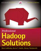
As shown in Figure 9-1, a common architecture for this type of implementation is very similar to a traditional database-based architecture, where HBase plays the role of traditional database(s). It is comprised of multiple load-balanced service implementations and a load balancer, which directs the client’s traffic to these implementations. A service implementation translates a client request into a sequence of read/write operations for HBase (and potentially additional data sources), combines and processes the data, and returns results back to the client.
FIGURE 9-1: Typical architecture for HBase-based application services
The main responsibilities of the service implementations in HBase-based real-time applications are similar to traditional service implementations, and include the following:
- Custom processing — A service provides a convenient place for custom data-processing logic, thus leveraging HBase-based (and potentially additional) data and application functionality.
- Semantic alignment — The implementation of service APIs enables you to align data in both content and granularity between what (and how) data is actually stored, and what an application is interested in. This provides a decoupling layer between an application’s semantics and the actual data storage.
- Performance improvements — The introduction of the services often improves overall performance because of the capability to implement multiple HBase gets/scans/puts locally, combine results, and send a single reply to the API consumer. (This assumes that the service implementation is co-located with the Hadoop cluster. Typically, these implementations are deployed either directly on Hadoop edge nodes, or, at least, on the same network segment as the Hadoop cluster itself.)
For the APIs exposed via the public Internet, you can implement an HBase-based real-time application by using REST APIs and leveraging one of the JAX-RS frameworks (for example, RestEasy or Jersey). If the APIs are used internally (say, within a company’s firewall), using the Avro RPC may be a more appropriate solution. In the case of REST (especially for large data sizes), you should still use Avro and binary payloads, which will often lead to better performance and better network utilization.
The remainder of this section examines two examples (using a picture-management system and using HBase as a Lucene back end) that demonstrate how you can build such real-time services while leveraging HBase. These examples show both the design approach to building such applications, and the implementation of the applications.
Using HBase as a Picture Management System
For the first example of a real-time Hadoop implementation, let’s take a look at a fictitious picture-management system. This system allows users to upload their pictures (along with the date when the pictures were taken), and then look up the pictures and download them based on the date.
Designing the System
Let’s start by designing data storage. Chapter 2 describes two basic data storage mechanisms provided by Hadoop:
- HDFS — This is used for storing large amounts of data while providing write, read, and append functionality with mostly sequential access.
- HBase — This is used for providing a full CRUD operations and random gets/scans/puts.
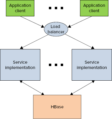
Chapter 2 also describes an approach for combining HDFS and HBase aimed at providing some of the HBase properties to large-sized data items. As shown in Figure 9-2, this is the approach used for this picture-management implementation.
FIGURE 9-2: Architecture for picture management system
For this example, let’s assume that every user is identified by a globally unique identifier (GUID), which is assigned to a user once he or she registers with the system. For each user, the system creates a directory containing SequenceFiles, which house the actual images uploaded by user. To simplify the overall design, let’s also assume that users are uploading their photos in bulk, and every bulk upload creates a new SequenceFile containing photographs that are part of this upload. Because different uploads can have radically different sizes, this approach can create a lot of “small” HDFS files, so it is necessary to implement a process that periodically combines smaller SequenceFiles into larger ones.
With this SequenceFile in place, the system will be able to store data fast. However, it will not provide a fast random access to pictures, which is typically required for picture-retrieval APIs. The APIs should support the return of a set of images for a given user for a given time interval.
To support the required access functionality, you must add an HBase-based index to the user’s pictures. You can do this by indexing all pictures for all users in a specialized HBase table — a picture index table. As shown in Listing 9-1, this table will have a key that contains a concatenation of the user’s Universally Unique Identification (UUID) and a timestamp for a picture that shows when the picture was taken.
LISTING 9-1: Picture management table key
UserUUID|Year|Mon|Day|Hour|Min|Sec Such a key design allows for a very efficient search for pictures for a given user for a given time interval, which is required for simple picture-retrieval APIs. A more complex, attribute-based search could be implemented by using a Lucene-based search, which is described later in this chapter.
The picture index table will contain one column family with one column name. Following the recommendations from Chapter 2 to keep these names short, you can use A as a column family name and B as a column name. The content of the column is the name of the SequenceFile (where the picture is stored), along with the byte offset from the beginning of the file.
With this high-level data design in place, the implementation is fairly straightforward. For an upload operation, a list of photographs from a given user is in the form of a timestamp, along with the byte array containing the image itself. At this point, a new SequenceFile is created and populated with the timestamp as a key, and the picture’s content as a value. When a new image is written to the file, its starting location (and the filename) are stored in the picture index table.
The read operations are initiated as a picture index table scan operation (for a given user and a date range). For every index found in the picture index table, an image is read from HDFS, based on the filename and offset. A list of pictures is then returned to the user.
You can also delete photographs by deleting a photograph from the index.
Finally, you can implement file compaction as a MapReduce job that is run periodically using an Oozie Coordinator (see Chapters 6 and 7 for more details on how to use Oozie Workflows and Coordinators), such as at midnight. For every user, this job scans the photograph’s index and rewrites the user’s photographs into a combined, sorted SequenceFile. This operation removes small files to improve HDFS utilization and overall system performance. (Pictures are stored in the timestamp order, thus avoiding additional seeks.) The operation also reclaims disk space by removing (not copying) deleted photographs.
Now, with the high-level design in place, let’s take a look at some of the actual implementation code.
Implementing the System
The implementation starts with the creation of a helper class shown in Listing 9-2 (code file: class DatedPhoto), which defines information that is used to send/receive a photo. Every image is accompanied by an epoch timestamp — that is, the number of milliseconds since January 1, 1970, 00:00:00.
LISTING 9-2: DatedPhoto class
public class DatedPhoto {

     long _date;
     byte[] _image;

     public DatedPhoto(){
          .........................
     }
     public DatedPhoto(long date, byte[] image){
          .........................
     }
     .........................................................................
     public static String timeToString(long time){
          .........................
     }
}
This is a fairly simple data container class. Not shown here are setters/getters. An additional method — timeToString — enables you to convert time from an epoch representation into a string representation, which is used in the table’s row key.
Another helper class shown in Listing 9-3 (code file: class PhotoLocation) defines index information saved for each image in HBase. This class also defines two additional methods — toBytes and fromBytes (remember, HBase stores all the values as byte arrays).
LISTING 9-3: PhotoLocation class
public class PhotoLocation implements Serializable{

     private long _pos;
     private long _time;
     private String _file;

     public PhotoLocation(){}

     public PhotoLocation(long time, String file, long pos){
          .........................
     }
     .........................................................................

     public byte[] toBytes(){
          .........................
          System.arraycopy(_pos, 0, _buffer, 0, 8);
          System.arraycopy(_time, 0, _buffer, 8, 8);
          System.arraycopy(_file, 0, _buffer, 16, _file.length());
          return _buffer;
     }

     public void fromBytes(byte[] buffer){
          System.arraycopy(buffer, 0, _pos, 0, 8);
          System.arraycopy(buffer, 8, _time, 0, 8);
          System.arraycopy(buffer, 16, _file, 0, buffer.length - 8);
     }
}
This is another data container class (getters/setters methods are omitted for brevity). toBytes()/fromBytes() methods in this class use a custom serialization/deserialization implementation. The custom implementation typically leads to a smallest size of binary data, but the creation of many custom implementations like this does not scale well as the number of classes grows.
With these two classes in place, you use a PhotoWriter class that is responsible for storage of the actual data to the SequenceFile. Then, index information for HBase can look like what is shown in Listing 9-4 (code file: class PhotoWriter).
LISTING 9-4: PhotoWriter class
public class PhotoWriter {

     private PhotoWriter(){}

     public static void writePhotos(UUID user, List<DatedPhoto> photos,
             String tName, Configuration conf) throws IOException{
          String uString = user.toString();
          Path rootPath = new Path(_root);
          FileSystem fs = rootPath.getFileSystem(conf);
          Path userPath = new Path(rootPath, uString);
          String fName = null;
          if(fs.getFileStatus(userPath).isDirectory()){
               FileStatus[] photofiles = fs.listStatus(userPath);
               fName = Integer.toString(photofiles.length);
          }
          SequenceFile.Writer fWriter = SequenceFile.createWriter(conf,................);
          HTable index = new HTable(conf, tName);
          PhotoLocation location = new PhotoLocation();
          location.setFile(fName);
          LongWritable sKey = new LongWritable();
          for(DatedPhoto photo : photos){
               long pos = fWriter.getLength();
               location.setPos(pos);
               location.setTime(photo.getLongDate());
               String key = uString + photo.getDate();
               sKey.set(photo.getLongDate());
               fWriter.append(sKey, new BytesWritable(photo.getPicture()));
               Put put = new Put(Bytes.toBytes(key));
               put.add(Bytes.toBytes("A"), Bytes.toBytes("B"), location.toBytes());
               index.put(put);
          }
          fWriter.close();
          index.close();
     }
     .........................................................
}
The writePhotos method first determines a new filename by querying a directory for a given user, calculating the number of files, and creating a name as a current length of this directory. It then creates a new SequenceFile writer and connects to a picture index (HBase) table. Once this is done, for every photo, a current file position is returned, and an image is added to the SequenceFile. Once an image is written, its index is added to the HBase table.
Listing 9-5 (code file: class PhotoDataReader) shows a helper class used for reading a specific photo (defined by an offset in the file) from a given file.
LISTING 9-5: PhotoDataReader class
public class PhotoDataReader {

     public PhotoDataReader(String file, UUID user, Configuration conf)
             throws IOException{

          _file = file;
          _conf = conf;
          _user = user.toString();
          _value = new BytesWritable();
          Path rootPath = new Path(PhotoWriter.getRoot());
          FileSystem fs = rootPath.getFileSystem(_conf);
          Path userPath = new Path(rootPath, _user);
          _fReader = new SequenceFile.Reader(fs, new Path(userPath, _file), _conf);
          _position = 0;
     }

     public byte[] getPicture(long pos) throws IOException{
          if(pos != _position)
               _fReader.seek(pos);
          boolean fresult = _fReader.next(_header, _value);
          if(!fresult)
               throw new IOException("EOF");
          _position = _fReader.getPosition();
          return _value.getBytes();
     }

     public void close() throws IOException{

          _fReader.close();
     }
}
The constructor of this class opens a SequenceFile reader for a given file, and positions the cursor at the beginning of the file. A getPicture method retrieves a picture, given its position in a file. To minimize the number of seeks, you first check if the file is in the right position (there is a high probability that pictures with adjacent indexes are located one after another), and seek only if the file is currently not at the required position. Once the file is at the right position, the method’s implementation reads the content of images, remembers the current position, and then returns an image.
Finally, Listing 9-6 (code file: class PhotoReader) shows a class that can be used to read either an individual photo, or a set of photos for a given time interval. This class also has an additional method to delete a picture with a given timestamp.
LISTING 9-6: PhotoReader class
public class PhotoReader {

     private PhotoReader(){}

     public static List<DatedPhoto> getPictures(UUID user, long startTime,
             long endTime, String tName,Configuration conf) throws IOException{

          List<DatedPhoto> result = new LinkedList<DatedPhoto>();
          HTable index = new HTable(conf, tName);
          String uString = user.toString();
          byte[] family = Bytes.toBytes("A");
          PhotoLocation location = new PhotoLocation();
          if(endTime < 0)
               endTime = startTime + 1;
          Map<String, PhotoDataReader> readers = new HashMap<String,
               PhotoDataReader>();
          Scan scan = new Scan(Bytes.toBytes(uString +
               DatedPhoto.timeToString(startTime)),
                    Bytes.toBytes(uString + DatedPhoto.timeToString(endTime)));
          scan.addColumn(family, family);
          Iterator<Result> rIterator = index.getScanner(scan).iterator();
          while(rIterator.hasNext()){
               Result r = rIterator.next();
               location.fromBytes(r.getBytes().get());
               PhotoDataReader dr = readers.get(location.getFile());
               if(dr == null){
                    dr = new PhotoDataReader(location.getFile(), user, conf);
                    readers.put(location.getFile(), dr);
               }
               DatedPhoto df = new DatedPhoto(location.getTime(),
                     dr.getPicture(location.getPos()));
               result.add(df);
          }
          for(PhotoDataReader dr : readers.values())
               dr.close();
          return result;
     }

     public static void deletePicture(UUID user, long startTime, String tName,
           Configuration conf) throws IOException{

          Delete delete = new Delete(Bytes.toBytes(user.toString() +
 DatedPhoto.timeToString(startTime)));
          HTable index = new HTable(conf, tName);
          index.delete(delete);
     }
}
The implementation of the read method first connects to the HBase table and creates a scan based on the input parameters. For every record returned by the scan, it first checks whether a PhotoDataReader for this filename already exists. If it does not, a new PhotoDataReader is created and added to the readers list. The reader is then used to obtain an image itself.
The implementation of the delete method just deletes photo information from the index table.
The solution presented here (in Listing 9-2 through Listing 9-6) provides a very rudimentary implementation of photo-management implementation, showing only a bare-bones Hadoop implementation. An actual implementation would be significantly more complex, but the code presented here illustrates a basic approach for building an HBase-based real-time system that could easily be extended for a real implementation.
The next example shows how to build an HBase-based back end for an inverted index, which can be used for an Hadoop-based real-time search.
Using HBase as a Lucene Back End
This significantly more realistic example describes an implementation of Lucene with an HBase back end that can be leveraged for real-time Hadoop-based search applications.
Overall Design
Before delving into HBase-based implementation, let’s start with a quick Lucene refresher. Lucene operates on searchable documents, which are collections of fields, each having a value. A field’s value is further comprised of one or more searchable elements — in other words, terms. Lucene search is based on an inverted index (refer to Chapter 3 for more about an inverted index and the algorithms for its calculations) that contains information about searchable documents. This inverted index allows for a fast look-up of a field’s term to find all the documents in which this term appears.
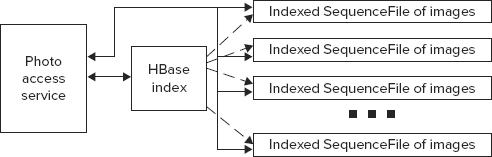
As shown in Figure 9-3, the following are the main components of the Lucene architecture:
FIGURE 9-3: High-level Lucene architecture
- IndexWriter calculates the reverse indexes for each inserted document and writes them out.
- IndexSearcher leverages IndexReader to read the inverted index and implement the search logic.
- Directory abstracts out the implementation of index data set access, and provides APIs (directly mimicking a file system API) for manipulating them. Both IndexReader and IndexWriter leverage Directory for access to this data.
At a very high level, Lucene operates on two distinct data sets, both of which are accessed based on an implementation of a Directory interface:
- The index data set keeps all the field/term pairs (with additional information such as term frequency, position, and so on), as well as the documents containing these terms, in appropriate fields.
- The document data set stores all the documents (including stored fields, and so on).
The standard Lucene distribution contains several Directory implementations, including filesystem-based and memory-based, Berkeley DB-based (in the Lucene contrib module), and several others.
The main drawback of a standard filesystem-based back end (Directory implementation) is a performance degradation caused by the index growth. Different techniques have been used to overcome this problem, including load balancing and index sharding (that is, splitting indexes between multiple Lucene instances). Although powerful, the use of sharding complicates the overall implementation architecture, and requires a certain amount of an a priori knowledge about expected documents before you can properly partition the Lucene indexes.
A different approach is to allow an index back end itself to shard data correctly, and then build an implementation based on such a back end. As described in Chapter 2, one such back-end storage implementation is HBase.
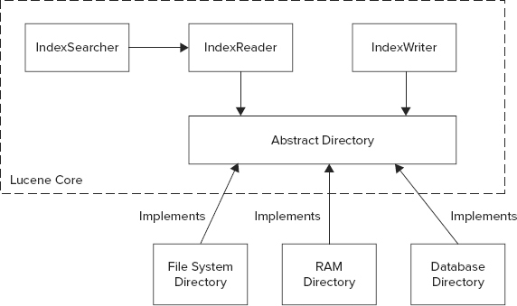
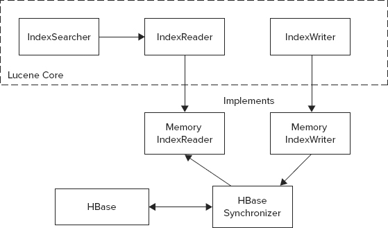
Because Lucene’s Directory APIs expose filesystem semantics, a “standard” way to implement a new Lucene back end is to impose such semantics on every new back end, which is not always the simplest (most convenient) approach to porting Lucene. As a result, several Lucene ports (including limited memory index support from the Lucene contrib module, Lucandra, and HBasene) took a different approach. As shown in Figure 9-4, these overwrote not a directory, but higher-level Lucene classes — IndexReader and IndexWriter — thus bypassing the Directory APIs.
FIGURE 9-4: Integrating Lucene with a back end without filesystem semantics

Although such an approach often requires more work, it also enables you to fully leverage the native capabilities of a particular back end. Consequently, it leads to significantly more powerful implementations. The implementation presented here follows this approach.
The overall implementation shown in Figure 9-5 is based on a memory-based back end that is used as an in-memory cache, along with a mechanism for synchronizing this cache with the HBase back end.
FIGURE 9-5: Overall architecture of HBase-based Lucene implementation
This implementation tries to balance two conflicting requirements — performance (the in-memory cache can drastically improve performance by minimizing the number of HBase reads for search and document retrieval) and scalability (the capability to run as many Lucene instances as required to support a growing population of search clients). The latter requires minimizing the cache lifetime to synchronize content with the HBase instance (that is, a single copy of truth). A compromise is achieved by implementing a configurable cache time-to-live (TTL) parameter, thus limiting cache presence in each Lucene instance.
- Sharded cache — Every CPU is dedicated to a specific portion of data. A given request is routed to a specific CPU, which is responsible for a portion of data that is cached locally. A cache eviction policy (if any) is least recently used (LRU).
- Random cache — Any CPU can service any request. The cache stores the results of the most recent requests. An eviction policy is necessary, and is typically least recently used (LRU) based on the amount of memory dedicated to the cache.
Both reads and writes (IndexReader/IndexWriter) are done through the memory cache, but their implementation is very different.
For reads, the cache first checks to see if the required data is in memory, and it is not stale (that is, has been in memory for too long). If both conditions are fulfilled, in-memory data is used. Otherwise, the cache reads/refreshes data from HBase, and then returns it to the IndexReader.
For writes, the data is written directly to HBase without storing it in memory. Although this might create a delay in actual data availability, it makes implementation significantly simpler — the writes can go to any Lucene instance without regard for the instance that might have a specific index value cached. To adhere to business requirements, the delay can be controlled by setting an appropriate cache expiration time.
This implementation is based on two main HBase tables — an index table and a document table.
As shown in Figure 9-6, the HBase index table, which is responsible for storing an inverse index, is the foundation of the implementation. This table has an entry (row) for every field/term combination (inverse key) known to a Lucene instance. Every row contains one column family (a “Documents family”). This column family contains a column (named as a document ID) for every document containing this field/term.
FIGURE 9-6: HBase index table
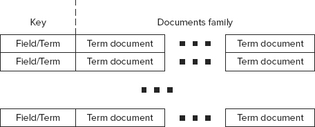
The content of each column is a value of TermDocument. The Avro schema for it is shown in Listing 9-7. (Chapter 2 provides more information about Avro.)
LISTING 9-7: TermDocument definition
{
  "type" : "record",
  "name" : "TermDocument",
  "namespace" : " com.practicalHadoop.lucene.document",
  "fields" : [ {
    "name" : "docFrequency",
    "type" : "int"
  }, {
    "name" : "docPositions",
    "type" : ["null", {
      "type" : "array",
      "items" : "int"
    }]
  } ]
}
As shown in Figure 9-7, the HBase document table stores documents themselves, back references to the indexes/norms, references to these documents, and some additional bookkeeping information used by Lucene for document processing. It has an entry (row) for every document known to a Lucene instance.
FIGURE 9-7: HBase document table
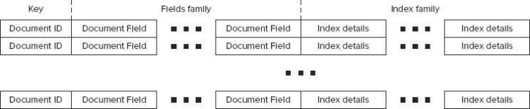
Each document is uniquely identified by a document ID (key) and contains two column families — the “Fields family” and the “Index family.” The Fields column family contains a column (named as a field name) for every field stored for a document. The column value shown in Listing 9-8 is comprised of the value type (string or byte array) and the value itself.
LISTING 9-8: Field definition
{
  "type" : "record",
  "name" : "FieldsData",
  "namespace" : " com.practicalHadoop.lucene.document",
  "fields" : [ {
    "name" : "fieldsArray",
    "type" : {
      "type" : "array",
      "items" : {
        "type" : "record",
        "name" : "singleField",
        "fields" : [ {
          "name" : "binary",
          "type" : "boolean"
        }, {
          "name" : "data",
          "type" : [ "string", "bytes" ]
        } ]
      }
    }
  } ]
}
The Index column family contains a column (named as a field/term) for every index referencing this document. The column value includes document frequency, positions, and offsets for a given field/term, as shown in Listing 9-9.
LISTING 9-9: TermDocumentFrequency
{
  "type" : "record",
  "name" : "TermDocumentFrequency",
  "namespace" : " com.practicalHadoop.lucene.document",
  "fields" : [ {
    "name" : "docFrequency",
    "type" : "int"
  }, {
    "name" : "docPositions",
    "type" : ["null",{
      "type" : "array",
      "items" : "int"
    }]
  }, {
    "name" : "docOffsets",
    "type" : ["null",{
      "type" : "array",
      "items" : {
        "type" : "record",
        "name" : "TermsOffset",
        "fields" : [ {
          "name" : "startOffset",
          "type" : "int"
        }, {
          "name" : "endOffset",
          "type" : "int"
        } ]
      }
    }]
  } ]
}As shown in Figure 9-8, an optional third table can be implemented if Lucene norms must be supported. The HBase norm table has an entry (row) for every field (key) known to the Lucene instance. Each row contains a single column family — the “Documents norms family.” This family has a column (named as document ID) for every document for which a given field’s norm must be stored.
FIGURE 9-8: HBase norm table

One of Lucene’s weakest points is spatial search. Although the Lucene spatial contribution package provides powerful support for spatial search, it is limited to finding the closest point. In reality, spatial search often has significantly more requirements, such as which points belong to a given shape (circle, bounding box, polygon), which shapes intersect with a given shape, and so on. As a result, the implementation presented here extends Lucene to solve such problems.
Geospatial Search
The geospatial search implementation for this example is based on a two-level search implementation:
- The first-level search is based on a Cartesian Grid search.
- The second level implements shape-specific spatial calculations.
For the Cartesian Grid search, the whole world is tiled at some zoom level. (Chapter 7 provides more about tiling and zoom levels.) In this case, a geometric shape is defined by the set of IDs of tiles that contain the complete shape. The calculation of these tile IDs is trivial for any shape type, and can be implemented in several lines of code.
In this case, both the document (referring to a certain shape) and the search shape can be represented by the list of tile IDs. This means that the first-level search implementation is just finding the intersection between tile IDs of the search shape and the document’s shape.
This can be implemented as a “standard” text search operation, which Lucene is very good at. Once the initial selection is done, geometrical arithmetic can be used to attain more precision by filtering the results of the first-level search. Such calculations can be as complex as they need to be to improve the precision of the search. These calculations are technically not part of the base implementation.
Figure 9-9 shows a concrete example. Here, only a limited number of tiles (1 through 12) and four documents (“a” through “e”) are shown.
FIGURE 9-9: Two-level search
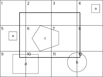
Based on its location and shape, each document can be described as a set of tile IDs — for example, “b” is contained in tiles 11 and 12. Now, let’s assume that you are searching for every document that intersects with a bounding box (represented by a wide line in Figure 9-9). As you can see, a search bounding box can be represented as a set of tiles with IDs 1 through 12. All shapes “a” through “e” will be found as a result of the first-level search. The second-level search will throw away shapes “a” and “e,” which do not intersect with the result bounding box. The overall search will return back shapes “b,” “c,” and “d.”
Incorporating this two-level algorithm into Lucene is fairly straightforward. The responsibility of Lucene’s engine is to support a first-level search — tile matching. The second-level search can be accomplished with external filtering, which does not necessarily need to be incorporated into Lucene.
To support both search levels, the Lucene document must be extended with the following additional fields:
- Shape field — This describes the shape associated with the document. (The current implementation is based on the serializable shape super class, and several specific shape implementations, including point, bounding box, circle, and polygon.) This can be used by the filter to obtain the shape with which the document is associated to perform explicit filtering.
- Tile ID field — This contains a field (or fields) describing the tile (or tiles) in which the shape is contained for different zoom levels.
Putting geospatial information directly into the document fields is the most simplistic approach for storing the geospatial information in a Lucene index. The drawback of such an approach is that it leads to the “explosion” of the index size (a new term/value must be created for every tile ID/zoom level combination), which will negatively impact HBase performance because of large row sizes.
As shown in Figure 9-10, a better approach is to store the document’s information for a given field/term value as multilevel hash tables.
FIGURE 9-10: Storing of geospatial indexes for a given field/term

The first level of this hash is determined by zoom level. For Level 1, the whole world is reserved for the requests without spatial information. This contains document information for all documents containing a given value for a given term. All other levels contain a hash map with document information for every document containing a given value for a given term, and located in a given tile ID. Because the number of documents contained in a given tile is always significantly smaller compared to the number of documents for the whole world, the search based on such an index organization is significantly faster than searches containing geospatial components, while preserving roughly the same search time for searches without them.
Although such an index organization can increase the required memory footprint, this increase will be relatively small because the overall implementation is based on the expiring lazy cache.
Technically, by introducing an additional keys structure, the original HBase table design shown in Figure 9-6 through Figure 9-8 can be used for storing multilevel hash tables.
Alternatively, as shown in Figure 9-11, to better cope with the significantly increased number of rows, and to further improve search scalability, instead of using a single HBase index table, N+1 index tables are introduced — one for global data, and one for every zoom level.
FIGURE 9-11: HBase index tables
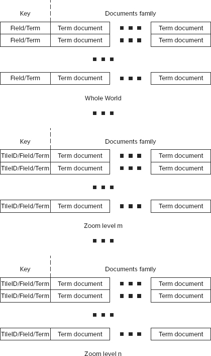
The whole world table shown in Figure 9-10 is exactly the same as an original index table shown in Figure 9-5, whereas tables for every zoom level have the same content, but a different key structure. For them, a key is a concatenation of not two, but three values — tile ID, field name, and term value.
In addition to the fact that splitting tables by zoom level enables you to make each table smaller (which simplifies overall HBase management), you can also add a parallelization of searches — requests for different zoom levels will read from different tables. The keys definition allows for natural support of scanning on the field/term level for a given zoom level/tile ID that is required by this Lucene implementation.
Now that you understand the overall design approach, let’s look at some of the implementation approaches — more specifically, the portion of implementation that is specific to Hadoop/HBase.
HBase Implementation Code
The example Lucene implementation requires access by multiple HBase tables several times during a search. Instead of creating and destroying a specific HTable class every time a table access is required (remember HTable class is not thread safe), the implementation leverages an HTablePool class (compare to database connection pooling). Listing 9-10 (code file: class TableManager) shows the class encapsulating HTablePool (TableManager), which additionally provides all configuration information (table names, family names, and so on).
LISTING 9-10: TableManager class
public class TableManager {

     // Levels
     private static final int _minLevel = 10;
     private static final int _maxLevel = 24;

     .....................................................................
     // Tables
     private static byte[] _indexTable;
     private static byte[][] _indexLevelTable;
     private static byte[] _documentsTable;
     private static byte[] _normsTable;

     //Families
     private static byte[] _indexTableDocuments;
     private static byte[] _documentsTableFields;
     private static byte[] _documentsTableTerms;
     private static byte[] _normsTableNorms;

     // Pool
     private HTablePool _tPool = null;
     private Configuration _config = null;
     private int _poolSize = Integer.MAX_VALUE;

     // Instance
     private static TableManager _instance = null;

     // Static initializer
     static{
          int nlevels = _maxLevel - _minLevel + 1;
          _indexLevelTable = new byte[nlevels][];
          _indexLevelTablePurpose = new String[nlevels];
          ..........................................................................

     }

     .....................................................................

     public static void setIndexTable(String indexTable, int level) {
          if(level < 0)
               _indexTable = Bytes.toBytes(indexTable);
          else{
               if((level >= _minLevel) && (level <= _maxLevel)){
                    int i = level - _minLevel;
                    _indexLevelTable[i] = Bytes.toBytes(indexTable);
               }
          }
     }

     .....................................................................

     public static synchronized TableManager getInstance()
                                             throws NotInitializedException{
          if(_instance == null)
               throw new NotInitializedException();
          return _instance;
     }


     private TableManager(Configuration config, int poolSize){

          if(poolSize > 0)
               _poolSize = poolSize;
          _config = config;
          _tPool = new HTablePool(_config, _poolSize);
     }

     public HTableInterface getIndexTable(int level) {

          if(level == 1)
               return _tPool.getTable(_indexTable);
          else
               return _tPool.getTable(_indexLevelTable[level-_minLevel]);
     }

     public HTableInterface getDocumentsTable(){

          return _tPool.getTable(_documentsTable);
     }

     public HTableInterface getNormsTable(){

          return _tPool.getTable(_normsTable);
     }

     public void releaseTable(HTableInterface t){

          try {
               t.close();
          } catch (IOException e) {}
     }
}
Because this class can support different numbers of levels, its static method allocates an array for table names for every level. The getTable methods in this class just get tables from the pool, while the releaseTable method returns tables back to the pool.
This example Lucene implementation uses several tables. A TableCreator class shown in Listing 9-11 (code file: class TableCreator) is based on HbaseAdmin APIs. It ensures that corresponding tables exist and are properly defined.
LISTING 9-11: TableCreator class
 public class TableCreator {

     public static List<HTable> getTables(TablesType tables, Configuration
             conf)throws Exception{

          HBaseAdmin hBaseAdmin = new HBaseAdmin(conf);
          List<HTable> result = new LinkedList<HTable>();
          for (TableType table : tables.getTable()) {
               HTableDescriptor desc = null;
               if (hBaseAdmin.tableExists(table.getName())) {
                    if (tables.isRebuild()) {
                         hBaseAdmin.disableTable(table.getName());
                         hBaseAdmin.deleteTable(table.getName());
                         createTable(hBaseAdmin, table);
                    }
                    else{
                         byte[] tBytes = Bytes.toBytes(table.getName());
                         desc = hBaseAdmin.getTableDescriptor(tBytes);
                         List<ColumnFamily> columns = table.getColumnFamily();
                       for(ColumnFamily family : columns){
                            boolean exists = false;
                            String name = family.getName();
                            for(HColumnDescriptor fm : desc.getFamilies()){
                                 String fmName = Bytes.toString(fm.getName());
                                 if(name.equals(fmName)){
                                      exists = true;
                                      break;
                                 }
                            }
                            if(!exists){
                                 System.out.println("Adding Famoly " + name + "
                                      to the table " + table.getName());
                                 hBaseAdmin.addColumn(tBytes,
                                      buildDescriptor(family));
                            }
                       }
                    }
               } else {
                    createTable(hBaseAdmin, table);
               }
               result.add( new HTable(conf, Bytes.toBytes(table.getName())) );
          }
          return result;
     }

     private static void createTable(HBaseAdmin hBaseAdmin,TableType table)
             throws Exception{
          HTableDescriptor desc = new HTableDescriptor(table.getName());
          if(table.getMaxFileSize() != null){
               Long fs = 1024l * 1024l *  table.getMaxFileSize();
               desc.setValue(HTableDescriptor.MAX_FILESIZE, fs.toString());
          }
          List<ColumnFamily> columns = table.getColumnFamily();
        for(ColumnFamily family : columns){
             desc.addFamily(buildDescriptor(family));
        }
        hBaseAdmin.createTable(desc);
     }

     private static HColumnDescriptor buildDescriptor(ColumnFamily family){

         HColumnDescriptor col = new HColumnDescriptor(family.getName());
         if(family.isBlockCacheEnabled() != null)
              col.setBlockCacheEnabled(family.isBlockCacheEnabled());
         if(family.isInMemory() != null)
              col.setInMemory(family.isInMemory());
         if(family.isBloomFilter() != null)
              col.setBloomFilterType(BloomType.ROWCOL);
         if(family.getMaxBlockSize() != null){
              int bs = 1024 * 1024 * family.getMaxBlockSize();
              col.setBlocksize(bs);
         }
         if(family.getMaxVersions() != null)
              col.setMaxVersions(family.getMaxVersions().intValue());
         if(family.getTimeToLive() != null)
              col.setTimeToLive(family.getTimeToLive());
         return col;
     }
}
This class is driven by an XML document that defines the required tables.
The helper method buildDescriptor builds an HColumnDescriptor based on the information provided by the XML configuration. The createTable method leverages the buildDescriptor method to build a table. Finally, the getTables method first checks whether the table exists. If it does, the method either deletes and re-creates it (if the rebuild flag is true), or adjusts it to the required configuration. If the table does not exist, then it just builds the table using the createTable method.
As discussed earlier, the two main table types used for implementation are IndexTable (as shown in Figure 9-10) and DocumentTable (as shown in Figure 9-6). Support for each type of table is implemented as a separate class providing all required APIs for manipulating data stored in the table.
Let’s start by looking at the IndexTableSupport class shown in Listing 9-12 (code file: class IndexTableSupport). As a reminder, this set of tables (one for each zoom level) stores all of the index information. Consequently, the IndexTableSupport class supports all index-related operations, including adding and removing a document to and from a given index, reading all documents for a given index, and removing the whole index.
LISTING 9-12: IndexTableSupport class
public class IndexTableSupport {

     private static TableManager _tManager = null;

     private IndexTableSupport(){}

     public static void init() throws NotInitializedException{
          _tManager = TableManager.getInstance();
     }

     ........................................................................
     public static void addMultiDocuments(Map<MultiTableIndexKey,
             Map<String,TermDocument>> rows, int level){

          HTableInterface index = null;

          List<Put> puts = new ArrayList<Put>(rows.size());
          try {
               for (Map.Entry<MultiTableIndexKey,
                       Map<String, TermDocument>> row : rows.entrySet()) {
                    byte[] bkey = Bytes.toBytes(row.getKey().getKey());
                    Put put = new Put(bkey);
                    put.setWriteToWAL(false);
                    for (Map.Entry<String, TermDocument> entry :
                            row.getValue().entrySet()) {
                         String docID = entry.getKey();
                         TermDocument td = entry.getValue();
                         put.add(TableManager.getIndexTableDocumentsFamily(),
                                   Bytes.toBytes(docID),
                                        AVRODataConverter.toBytes(td));
                    }
                    puts.add(put);
               }
               for(int i = 0; i < 2; i++){
                    try {
                         index = _tManager.getIndexTable(level);
                         index.put(puts);
                         break;
                    } catch (Exception e) {
                         System.out.println("Index Table support. Reseting pool
                              due to the multiput exception ");
                         e.printStackTrace();
                         _tManager.resetTPool();
                    }
               }
          } catch (Exception e) {
               e.printStackTrace();
          }
          finally{
               _tManager.releaseTable(index);
          }
     }

     public static void deleteDocument(IndexKey key, String docID)throws Exception{

          if(_tManager == null)
               throw new NotInitializedException();
          HTableInterface index = _tManager.getIndexTable(key.getLevel());
          if(index == null)
               throw new Exception("no Table");
          byte[] bkey = Bytes.toBytes(new MultiTableIndexKey(key).getKey());
          byte[] bID = Bytes.toBytes(docID);
          Delete delete = new Delete(bkey);
          delete.deleteColumn(TableManager.getIndexTableDocumentsFamily(), bID);
          try {
               index.delete(delete);
          } catch (Exception e) {
               throw new Exception(e);
          }
          finally{
               _tManager.releaseTable(index);
          }
     }

     public static void deleteIndex(IndexKey key)throws Exception{

          if(_tManager == null)
               throw new NotInitializedException();
          HTableInterface index = _tManager.getIndexTable(key.getLevel());
          if(index == null)
               throw new Exception("no Table");
          byte[] bkey = Bytes.toBytes(new MultiTableIndexKey(key).getKey());
          Delete delete = new Delete(bkey);
          try {
               index.delete(delete);
          } catch (Exception e) {
               throw new Exception(e);
          }
          finally{
               _tManager.releaseTable(index);
          }
     }

     public static TermDocuments getIndex(IndexKey key)throws Exception{

          if(_tManager == null)
               throw new NotInitializedException();
          HTableInterface index = _tManager.getIndexTable(key.getLevel());
          if(index == null)
               throw new Exception("no Table");
          byte[] bkey = Bytes.toBytes(new MultiTableIndexKey(key).getKey());
          try {
               Get get = new Get(bkey);
               Result result = index.get(get);
               return processResult(result);
          } catch (Exception e) {
               throw new Exception(e);
          }
          finally{
               _tManager.releaseTable(index);
          }
     }

     ...................................................................................................

     private static TermDocuments processResult(Result result)throws Exception{

          if((result == null) || (result.isEmpty())){
               return null;
          }

          Map<String, TermDocument> docs = null;
          NavigableMap<byte[], byte[]> documents =
               result.getFamilyMap
               (TableManager.getIndexTableDocumentsFamily());
          if((documents != null) && (!documents.isEmpty())){
               docs = Collections.synchronizedMap(new HashMap<String,
                    TermDocument>(50, .7f));
               for(Map.Entry<byte[], byte[]> entry : documents.entrySet()){
                    TermDocument std = null;
                    try {
                         std = AVRODataConverter.unmarshallTermDocument
                              (entry.getValue());
                    } catch (Exception e) {
                         System.out.println("Barfed in Avro conversion");
                         e.printStackTrace();
                         throw new Exception(e);
                    }
                    docs.put(Bytes.toString(entry.getKey()), std);
               }
          }
          return docs == null ? null : new TermDocuments(docs);
     }
     ...........................................................................................
}
The implementation of the addMultiDocuments method is fairly straightforward. To optimize HBase write performance, it is leveraging multi-PUTs (see the discussion on the HBase PUT performance in Chapter 2). So, it is first building a list of PUTs for all documents that must be added to the index, and then writing all of them to HBase. Note the retry mechanism used in this method. The implementation tries to retry several times, each time resetting the pool to ensure that no stale HBase connections exist.
The deleteDocument and deleteIndex methods are using the HBase delete command for a given column and a complete row, respectively.
Finally, the getIndex method is reading information about all the documents for a given index. It is using a simple HBase Get command to get the complete row, and then uses the processResult method to convert the result to a map of TermDocument objects. Both addMultiDocuments and getIndex methods are leveraging Avro to convert data to and from a binary representation.
The DocumentTableSupport class shown in Listing 9-13 (code file: class DocumentTableSupport) supports all document-related operations, including adding, retrieving, and removing documents.
LISTING 9-13: DocumentTableSupport class
public class DocumentsTableSupport {

     private static TableManager _tManager = null;

     private DocumentsTableSupport(){}

     public static void init() throws NotInitializedException{
          _tManager = TableManager.getInstance();
     }

     .......................................................................
     public static void addMultiDocuments(DocumentCollector collector){

          HTableInterface documents = null;
          Map<String, DocumentInfo> rows = collector.getRows();
          List<Put> puts = new ArrayList<Put>(rows.size());
          try {
               for(Map.Entry<String, DocumentInfo> row : rows.entrySet()){
                    byte[] bkey = Bytes.toBytes(row.getKey());
                    Put put = new Put(bkey);
                    put.setWriteToWAL(false);
                    for(Map.Entry<String, FieldsData> field :
                            row.getValue().getFields().entrySet())
                         put.add(TableManager.getDocumentsTableFieldsFamily(),
                              Bytes.toBytes(field.getKey()),
                              AVRODataConverter.toBytes(field.getValue()));
                    for(Map.Entry<IndexKey, TermDocumentFrequency> term :
                            row.getValue().getTerms().entrySet())
                         put.add(TableManager.getDocumentsTableTermsFamily(),
                              Bytes.toBytes(term.getKey().getKey()),
                              AVRODataConverter.toBytes(term.getValue()));
                    puts.add(put);
               }
               for(int i = 0; i < 2; i++){
                    try {
                         documents = _tManager.getDocumentsTable();
                         documents.put(puts);
                         break;
                    } catch (Exception e) {
                         System.out.println("Documents Table support. Reseting
                              pool due to the multiput exception ");
                         e.printStackTrace();
                         _tManager.resetTPool();
                    }
               }
          } catch (Exception e) {
               e.printStackTrace();
          }
          finally{
               _tManager.releaseTable(documents);
          }
     }

     public static List<IndexKey> deleteDocument(String docID)throws Exception{

          if(_tManager == null)
               throw new NotInitializedException();
          HTableInterface documents = _tManager.getDocumentsTable();
          byte[] bkey = Bytes.toBytes(docID);

          List<IndexKey> terms;
          try {
               Get get = new Get(bkey);
               Result result = documents.get(get);
               if(result == null){     // Does not exist
                    _tManager.releaseTable(documents);
                    return null;
               }
               NavigableMap<byte[], byte[]> data =
                    result.getFamilyMap
                    (TableManager.getDocumentsTableTermsFamily());
               terms = null;
               if((data != null) && (!data.isEmpty())){
                    terms = new LinkedList<IndexKey>();
                    for(Map.Entry<byte[], byte[]> term : data.entrySet())
                         terms.add(new IndexKey(term.getKey()));
               }
               Delete delete = new Delete(bkey);
               documents.delete(delete);
               return terms;
          } catch (Exception e) {
               throw new Exception(e);
          }
          finally{
               _tManager.releaseTable(documents);
          }
     }

     ................................................................................

     public static List<DocumentInfo> getDocuments(List<String> docIDs)throws
             Exception{

          if(_tManager == null)
               throw new NotInitializedException();
          HTableInterface documents = _tManager.getDocumentsTable();
          List<Get> gets = new ArrayList<Get>(docIDs.size());
          for(String docID : docIDs)
               gets.add(new Get(Bytes.toBytes(docID)));
          List<DocumentInfo> results = new ArrayList<DocumentInfo>(docIDs.size());
          try {
               Result[] result = documents.get(gets);
               if((result == null) || (result.length < 1)){
                    for(int i = 0; i < docIDs.size(); i++)
                         results.add(null);
               }
               else{
                    for(Result r : result)
                         results.add(processResult(r));
               }
               return results;
          } catch (Exception e) {
               throw new Exception(e);
          }
          finally{
               _tManager.releaseTable(documents);
          }
     }

     private static DocumentInfo processResult(Result result) throws Exception{

          if((result == null) || (result.isEmpty())){
               return null;
          }
          Map<String, FieldsData> fields = null;
          Map<IndexKey, TermDocumentFrequency> terms = null;
          NavigableMap<byte[], byte[]> data =
                  result.getFamilyMap
                  (TableManager.getDocumentsTableFieldsFamily());
          if((data != null) && (!data.isEmpty())){
               fields = Collections.synchronizedMap(new HashMap<String,
                       FieldsData>(50, .7f));
               for(Map.Entry<byte[], byte[]> field : data.entrySet()){
                    fields.put(Bytes.toString(field.getKey()),
                            AVRODataConverter.unmarshallFieldData
                            (field.getValue()));
               }
          }
          data = result.getFamilyMap(TableManager.getDocumentsTableTermsFamily());
          if((data != null) && (!data.isEmpty())){
               terms = Collections.synchronizedMap(new HashMap<IndexKey,
                    TermDocumentFrequency>());
               for(Map.Entry<byte[], byte[]> term : data.entrySet()){
                    IndexKey key = new IndexKey(term.getKey());
                    byte[] value = term.getValue();
                    TermDocumentFrequency tdf =
                         AVRODataConverter.unmarshallTermDocumentFrequency
                         (value);
                    terms.put(key, tdf);
               }
          }
          return new DocumentInfo(terms, fields);
     }
     ......................................................................................................................
}
Implementation of this class is similar to the implementation of the IndexTableSupport class. It implements similar methods and employs the same optimization techniques.
Now that you know how to use HBase for building real-time Hadoop implementations, let’s take a look at a new growing class of specialized Hadoop applications — specialized real-time Hadoop queries.
USING SPECIALIZED REAL-TIME HADOOP QUERY SYSTEMS
One of the first real-time Big Data query implementations was introduced by Google in 2010. Dremel is a scalable, interactive, ad-hoc query system used to analyze read-only nested data. The foundation of Dremel is as follows:
- Dremel represents an implementation of a novel columnar storage format for nested relational data/data with nested structures that was largely introduced in the article, “Column Oriented Storage Techniques for MapReduce” by Avrilia Floratou, Jignesh M. Patel, Eugene J. Shekita, and Sandeep Tata (published by Very Large Data Base Endowment, also known as VLDB, in 2011). The article introduced a format itself, its integration with HDFS, and a “skip list” approach to reading only required data, thus allowing you to significantly improve the performance of conditional reads.
- Dremel uses distributed scalable aggregation algorithms, which allow the results of a query to be computed on thousands of machines in parallel.
A columnar storage model shown in Figure 9-12 originates from flat relational data, and is extended to support nested data model. This model contains several fields — A, B, C, D, and E. Fields C, D, and E each have records r1 and r2, while fields A and B have no records, but contain related fields. In this model, all nested fields (B, C, D, and E) are stored continuously. Two main techniques can then be used to optimize read performance:
FIGURE 9-12: Column-oriented storage in Dremel
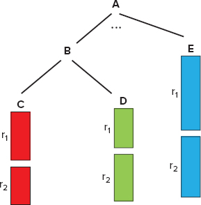
- Skip lists (for example, if sequential layout is A, B, C, D, E, and only A and E are required, after reading A, you can skip B, C, and D, and jump directly to E)
- Lazy deserialization (that is, keeping data as a binary blob until serialization is required)
Figure 9-13 shows the implementation of a distributed scalable query that leverages Dremel’s multilevel serving tree architecture. The incoming client requests come to the root server, which routes requests to the intermediate servers based on request types. There can be several layers of intermediate servers with their own routing rules. The leaf servers use a storage layer (based on the columnar storage model described earlier) to read the required data (which is bubbling up for aggregation), and the final result is returned to the user.
FIGURE 9-13: Dremel overall architecture

Overall, Dremel combines parallel query execution with the columnar format, thus supporting high-performance data access.
As Hadoop’s popularity and adoption grow, more people will be using its storage capabilities. As a result, specialized real-time query engines are currently a source of competition among Hadoop vendors and specialized companies. As of this writing, there are several Hadoop projects that have been inspired by Dremel:
- Open Dremel is currently part of Apache Drill (an Apache Incubator project since 2012).
- Cloudera introduced Impala (currently in beta state), which is part of the Cloudera Hadoop distribution (CDH 4.1). (There are also plans to either move this to Apache, or use an Apache license and make it available as a GitHub project.)
- The Stinger Initiative was introduced by Hortonworks in 2013 (real-time Hive). It has been submitted to Apache’s incubation process.
- HAWQ is part of a version of Greenplum’s Hadoop distribution — Pivotal HD.
Currently, real-time Hadoop queries represent a “bleeding edge” of Hadoop development. Many believe that such implementations will be new “killer” Hadoop applications by combining the power of Hadoop storage with the pervasive use of SQL. Such systems can also provide an easy path for integration between Hadoop and modern business intelligence (BI) tools, thus simplifying the bringing of Hadoop-based data to a wider audience.
All implementations are in various stages of maturity. For this discussion, let’s take a look at the two that have been around the longest — Drill and Impala.
Apache Drill
As of this writing, Drill is a very active Apache incubating project led by MapR with six to seven companies actively participating, and more than 250 people currently on the Drill mailing list.
The goal of Drill is to create an interactive analysis platform for Big Data using a standard SQL-supporting relational database management system (RDBMS), Hadoop, and other NoSQL implementations (including Cassandra and MongoDB).
As shown in Figure 9-14, the foundation of the Drill architecture is a set of Drillbits processes — that is, Drill executables running on Hadoop’s DataNodes to provide data locality and parallel query execution.
FIGURE 9-14: Overall Drill architecture
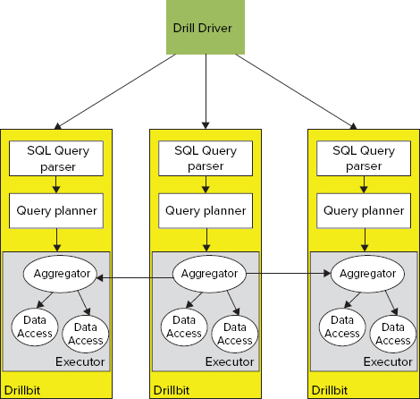
An individual query request can be delivered to any of the Drillbits. It is first processed by a SQL query parser, which parses the incoming query and passes it to the co-located query planner.
The SQL query planner provides query optimization. A default optimizer is a cost-based optimizer, but additional custom optimizers can be introduced, based on the open APIs provided by Drill.
Once a query plan is ready, it is processed by a set of distributed executors. A query execution is spread between multiple DataNodes in order to support data locality. Execution of a query on a particular data set is done on the node where the data is located. Additionally, to improve the overall performance, results of queries for local data sets are aggregated locally, and only combined query results are returned back to the executor that started a query.
Drill’s query parser supports full SQL (ANSI SQL:2003), including correlated sub-query, analytics functions, and so on. In addition to standard relational data, Drill supports (using ANSI SQL extensions) hierarchical data, including XML, JavaScript Object Notation (JSON), Binary JSON (BSON), Avro, protocol buffers, and so on.
Drill also supports dynamic data schema discovery (schema-less queries). This feature is especially important when dealing with NoSQL databases, including HBase, Cassandra, MongoDB, and so on, where every record can effectively have a different schema. It also simplifies support for schema evolution.
Finally, the SQL parser supports custom domain-specific SQL extensions based on User Defined Functions (UDFs), User Defined Table Functions (UDTFs), and custom operators (for example, Mahout’s k-means operator).
Whereas Drill is, for the most part, still in a development state, the other specialized Hadoop query language implementation — Impala — is currently available for initial experimentation and testing. Let’s take a closer look at the details of Impala implementation.
Impala
Impala (which was in beta version at the time of this writing) is one of the first open source implementations of real-time Hadoop query systems. Although technically an open source (GitHub) project, Impala currently requires a specific Hadoop installation (CDH4.2 for the latest Impala version).
An Impala implementation makes use of some of the existing Hadoop infrastructure, namely the Hive metastore and Hive ODBC driver. Impala operates on Hive tables and uses HiveQL as a query language.
- Data Definition Language (DDL) such as CREATE, ALTER, and DROP (although it can be implemented using a Hive shell)
- LOAD DATA to load raw files (although it can be implemented using a Hive shell)
- Non-scalar data types such as maps, arrays, and structs
- XML and JSON functions
- Extensibility mechanisms such as TRANSFORM, custom UDFs, custom file formats, or custom serialization/deserealization (SerDes)
- User Defined Aggregate Functions (UDAFs)
- User Defined Table Generating Functions (UDTFs)
- Sampling
Figure 9-15 shows Impala’s architecture. As shown in the figure, the process is as follows:
FIGURE 9-15: Impala overall architecture
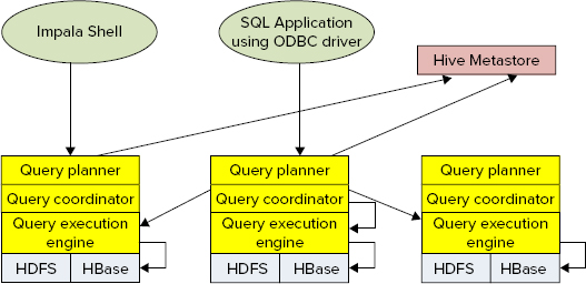
The current version of Impala supports both HDFS and HBase data storage. File formats currently supported for HDFS include TextFile, SequenceFile, RCFile, and Avro. Support for a new columnar format (Trevini) has been advertised by Cloudera.
HBase support is based on mapping a Hive table to HBase. This mapping can be done either based on a primary key (for best performance), or any other column (using a full table to scan with SingleColumnValueFilter, which can cause a significant performance degradation, especially for large tables).
Access for both HDFS and HBase supports several compression codecs, including Snappy, GZIP, Deflate, and BZIP.
In addition to its own shell, Impala supports Hive’s user interface (Hue Beeswax).
Now that you are familiar with Hadoop’s real-time queries and some of their implementations, let’s see how the real-time query system stacks up against MapReduce.
Comparing Real-Time Queries to MapReduce
Table 9-1 summarizes the main differences between real-time query systems and MapReduce. This table can help you decide on which type of system you should base your implementation.
TABLE 9-1: Key Differences between Real-Time Query System and MapReduce
| KEY DIFFERENCES | REAL-TIME QUERY ENGINES | MAPREDUCE |
| Purpose | Query service for large data sets | Programming model for processing large data sets |
| Usage | Ad hoc and trial-and-error interactive query of large data sets for quick analysis and troubleshooting | Batch processing of large data sets for time-consuming data conversion or aggregation |
| OLAP/BI use case | Yes | No |
| Data mining use case | Limited | Yes |
| Programming complex data processing logic | No | Yes |
| Processing unstructured data | Limited (regular expression matching on text) | Yes |
| Handling large results/join large table | No | Yes |
Now that you know about specialized real-time Hadoop query systems, let’s look at another fast-growing set of real-time Hadoop-based applications — event processing.
USING HADOOP-BASED EVENT-PROCESSING SYSTEMS
Event processing (EP) systems enable you to track (in real time) and process continuous streams of data. Complex event processing (CEP) systems support holistic processing of data from multiple sources.
Considering Hadoop’s capability to store massive amounts of data such as what can be produced by CEP systems, Hadoop seems like a good fit for large-scale CEP implementations.
A common implementation architecture for a CEP system is known as an actor model. In this case, every actor is responsible for partial processing of a certain event. (Mapping events to actors can be implemented in different ways, based on the event types, a combination of event types, and some additional attributes.) When an actor is finished with the processing of incoming events, it can send results for further processing to other actors. Such an architecture provides for a very clean componentization of the overall processing, and encapsulates certain processing logic.
- Make local decisions
- Create more actors
- Send messages
- Determine how to respond to the next received message
Once the actor’s implementation is in place, the overall system’s responsibility is to manage the actor’s life cycle and communications between actors.
Although CEP in general is a fairly mature architecture with quite a few established implementations, usage of Hadoop for CEP is relatively new and is not quite mature enough. Two different approaches to implementing CEP-based Hadoop systems exist:
- Modifying a MapReduce execution to accommodate event-processing needs. Examples of such systems include HStreaming and HFlame.
- “Hadoop-like” CEP implementations, which use a range of Hadoop technologies and can be integrated with Hadoop to leverage its data storing capabilities. Examples of such systems include Storm, S4, and so on.
HFlame
As explained in Chapter 3, MapReduce operates on key/value pairs, as shown in Figure 9-16. A mapper takes input in the form of key/value pairs (k1, v1) and transforms them into another key/value pair (k2, v2). The framework sorts the mapper’s output key/value pairs and combines each unique key with all its values (k2, {v2, v2,...}). These key/value combinations are delivered to reducers, which translate them into yet another key/value pair (k3, v3).
FIGURE 9-16: MapReduce processing

The basic difference between MapReduce processing and the actor model is the fact that the actor model operates on “live” data streams, whereas MapReduce operates on data already stored in Hadoop. Additionally, MapReduce mappers and reducers are instantiated specifically for executing a specific job, which makes MapReduce too slow for real-time event processing.
HFlame is an Hadoop’s extension that attempts to improve basic MapReduce performance by providing support for long-running mappers and reducers, which processes the new contents as soon as they are stored in HDFS.
Figure 9-17 shows the overall architecture of HFlame working in this mode.
FIGURE 9-17: HFlame overall architecture
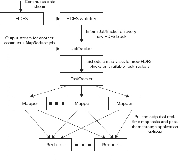
In this case, once the data is written to HDFS, a data watcher (HDFS watcher) invokes a MapReduce JobTracker, informing it about the availability of a new data. A JobTracker checks with the TaskTrackers to find an available map task, and passes data to it. Once the map method is complete, the data is sent to the appropriate reducer.
An output of an HFlame continuous job can be further represented as a continuous stream of data, which can be consumed by another MapReduce job running in continuous mode. This execution chaining mechanism allows pipelines of arbitrary complexity to be built (similar to chaining MapReduce jobs, described in Chapter 3).
Although implementation of the actor model in HFlame is quite simple, it often violates one of the principles of functional programming, which is a base MapReduce execution model. The problem is that the majority of implementations of actors are stateful (compared to the in-memory combiner pattern, described in Chapter 4). This means that every actor keeps internal memory for its execution, and you should carefully choose the number of reducers to ensure that a reducer process has enough memory to accommodate all active actors.
Another issue is the fact that, in the case of a reducer’s failure, Hadoop will restart the process, but the state of the actors (kept in memory) disappears. This typically is not a problem for a large-scale CEP system that is processing millions of requests, but something that requires careful designing and planning.
The way to get around these problems is to create a persistence layer for an actor’s state that can, for example, leverage HBase. However, such an implementation adds latency (with an HBase read prior to actor execution, and one write immediately after) and complexity. But this can make the overall implementation significantly more robust.
The HFlame distribution comes with several CEP examples, including fraud detection for the financial industry, failure/fault detection for the telecommunications and energy industries, continuous insights for Facebook and Twitter, and so on.
Now let’s take a look at an Hadoop-like CEP system using Storm as an example, and see how it works.
Storm
Storm is a new real-time event processing system that is distributed, reliable, and fault-tolerant. Storm (sometimes called “Hadoop for stream processing”) is not really Hadoop, but leverages many Hadoop ideas, principles, and some Hadoop sub-projects. You can integrate it with Hadoop for storing processing results that can later be analyzed using Hadoop tools.
Figure 9-18 shows the overall Storm architecture. You will notice a lot of commonalities between MapReduce and Storm architectures. Storm’s overall execution is controlled by a master process — Nimbus. It is responsible for distributing code around the cluster, assigning tasks to machines, and monitoring for failures. A lot of commonalities exist between the functionality of Nimbus and of the MapReduce JobTracker. Similar to the JobTracker, Nimbus is running on a separate control node, which is called a master in Storm.
FIGURE 9-18: Storm high-level architecture

All other nodes in the Storm cluster are worker nodes that run one specialized process — Supervisor. The role of the Supervisor is to manage resources on a particular machine (compared to the MapReduce TaskTracker). Supervisor accepts requests for work from Nimbus. It starts and stops local worker processes based on these requests.
Unlike a MapReduce implementation where TaskTrackers monitor a heartbeat directly to the JobTracker (which directly keeps track of the cluster topology), Storm uses a Zookeeper cluster (see Chapter 2 for additional information on Zookeeper) for coordination between master and worker nodes. An additional role of Zookeeper in Storm is to keep state for both Nimbus and Supervisor. This allows both to be stateless, which leads to a very fast recovery of any Storm node. Both Nimbus and Supervisor are implemented to fail fast, which, coupled with fast recovery, leads to a high stability of Storm clusters.
Unlike MapReduce (which operates on a finite number of key/value pairs), Storm operates on streams of events — or an unbounded sequence of tuples. As shown in Figure 9-19, Storm applications (or topologies) are defined in the form of input streams (called spouts) and a connected graph of processing nodes (called bolts).
FIGURE 9-19: Storm application

Spouts typically read data tuples from the external source, and emit them into a topology. Spouts can be reliable (for example, replaying a tuple that failed to be processed) and unreliable. A single spout can produce more than one stream.
Bolts are processing workhorses of Storm. They are similar to actors in the actor model. Bolts can do anything from filtering, functions, aggregations, joins, talking to databases, to emitting streams, and more. Bolts can do simple data transformations. Doing complex stream transformations often requires multiple steps, and, thus, chaining bolts (compare this with MapReduce jobs chaining).
The bolt chaining-processing dependency execution (compare this with DAG of MapReduce jobs defined by Oozie) is defined by Storm’s topology — that is, a Storm application. The topology is created in Storm using a topology builder.
The routing of tuples between bolts in Storm is accomplished by using stream grouping. Stream grouping defines how specific tuples are sent from one bolt to another. Storm comes with several prebuilt stream groupings, including the following:
- Shuffle grouping — This provides a random distribution of tuples between the bolts in a way that guarantees that each bolt will get an equal number of tuples. This type of grouping is useful for load balancing between identical stateless bolts.
- Fields grouping — This provides a partitioning of a stream based on fields specified in the grouping. This type of grouping guarantees that the tuples with the same field(s) value will always go to the same bolt, while tuples with different field value(s) may go to different bolts. This grouping is similar to MapReduce’s shuffle and sort processing, guaranteeing that a map’s outputs with the same keys will always go to the same reducer. This type of grouping is useful for implementation of stateful bolts, such as counters, aggregators, joins, and so on.
- All grouping — This replicates stream values across all participating bolt tasks.
- Global grouping — This allows an entire stream to go to a single bolt (a bolt with the lowest ID is used in this case). This type of grouping is equivalent to a MapReduce job with a single reducer, and is useful for implementing global counters, top N, and so on.
- Direct grouping — This allows a tuple producer to explicitly pick a tuple’s destination. This type of grouping requires a tuple emitter to know the IDs of participating bolts, and is restricted to a special type of streams — direct streams.
- Local or shuffle grouping — This ensures that, if possible, a tuple will be delivered within a local process. If the target bolt does not exist in the current process, this acts as a normal shuffle grouping. This type of grouping is often used for optimizing execution performance.
Additionally, Storm enables developers to implement custom stream grouping.
A topology is packaged in a single jar file that is submitted to a Storm cluster. This jar contains a class with main function that defines the topology to be submitted to Nimbus. Nimbus analyzes the topology and distributes parts of it to the Supervisors, which are responsible for starting, executing, and stopping worker processes, as necessary, for execution of the given topology.
Storm provides a very powerful framework for execution of various real-time applications. Similar to MapReduce, Storm provides a simplified programming model, which hides the complexity of implementing a long-running distributed application, and allows developers to concentrate on a business-processing implementation, while providing all complex infrastructure plumbing.
Now that you are familiar with Hadoop-based event processing and some implementations, let’s see how it stacks up against MapReduce.
Comparing Event Processing to MapReduce
Table 9-2 summarizes the main differences between event-processing systems and MapReduce. This can serve as a guide to help you decide on which type of system to base your implementation.
TABLE 9-2: Key Differences between Event-Processing System and MapReduce
| KEY DIFFERENCES | EVENT PROCESSING | MAPREDUCE |
| Purpose | Filter, correlate, and process events in real time | Programming model for processing large data sets |
| Usage | An environment for development and deployment of event-processing applications that can process and act on hundreds or thousands of events per second | Batch processing of large data sets for time-consuming data conversion or aggregation |
| Deployment | Separate (predefined) | Just in time (in code) |
| Real-time, event-driven applications | Yes | No |
| Programming complex data processing logic | Yes | Yes |
| Processing unstructured data | Limited | Yes |
SUMMARY
In this chapter, you have learned about different approaches to implementing Hadoop-based real-time applications, and the underlying architectural principles behind such implementations.
You also learned how HBase can be leveraged for building Hadoop-based real-time applications. You learned about the design and implementation of two sample applications — a picture-management system, and an HBase-based Lucene back end. Both applications demonstrate how such implementations can be designed, and the role HBase plays in the overall implementation.
This chapter also introduced you to two very active areas of Hadoop development — real-time SQL query systems and Hadoop-based event-processing systems. You learned about the base architecture of such systems, and their overall capabilities. You also learned how such systems can be compared to MapReduce, and what you should consider when choosing a particular implementation.
Now that you have learned different techniques and technologies for development of Hadoop-based applications, Chapter 10 shows you how to secure these applications.