2 Differential privacy for machine learning

This chapter covers

• What differential privacy is
• Using differential privacy mechanisms in algorithms and applications
• Implementing properties of differential privacy

In the previous chapter, we investigated various privacy-related threats and vulnerabilities in machine learning (ML) and concepts behind privacy-enhancing technologies. From now on, we will focus on the details of essential and popular privacy-enhancing technologies. The one we will discuss in this chapter and the next is differential privacy (DP).

Differential privacy is one of the most popular and influential privacy protection schemes used in applications today. It is based on the concept of making a dataset robust enough that any single substitution in the dataset will not reveal any private information. This is typically achieved by calculating the patterns of groups within the dataset, which we call complex statistics, while withholding information about individuals in the dataset.

For instance, we can consider an ML model to be complex statistics describing the distribution of its training data. Thus, differential privacy allows us to quantify the degree of privacy protection provided by an algorithm on the (private) dataset it operates on. In this chapter, we’ll look at what differential privacy is and how it has been widely adopted in practical applications. You’ll also learn about its various essential properties.

2.1 What is differential privacy?

Many modern applications generate a pile of personal data belonging to different individuals and organizations, and there are serious privacy concerns when this data leaves the hands of the data owners. For instance, the AOL search engine log data leak [1] and Netflix recommendation contest privacy lawsuit [2] show the threats and the need for rigorous privacy-enhancing techniques for ML algorithms. To address these challenges, differential privacy (DP) has evolved as a promising privacy-enhancing technique that provides a rigorous definition of privacy [3], [4].

2.1.1 The concept of differential privacy

Before introducing the definition of differential privacy, let’s look at an example, which is illustrated in figure 2.1.

Figure 2.1 The problem of personal information leakage

Suppose Alice and Bob are news reporters from different news agencies who wanted to report on the average salary of a private company. This company has a database containing the personal information of all its employees (such as position, wages, and contacts). Since the database includes personal data subject to privacy concerns, direct access to the database is restricted. Alice and Bob were required to demonstrate that they planned to follow the company’s protocols for handling personal data by undergoing confidentiality training and signing data use agreements proscribing the use and disclosure of personal information obtained from the database. The company granted Alice and Bob access to query certain aggregated statistics from the company’s database, including the total number of employees and the average salaries, but not to access any personal information, such as name or age.

In January 2020, Alice wrote an article based on the information obtained from that database, reporting that the private company has 100 employees, and the average salary is $55,000. In February 2020, Bob wrote an article based on the information he obtained from the database in the same way, reporting that the private company has 101 employees, and the average salary is $56,000. The only difference is that Alice accessed the database in January, whereas Bob accessed it in February.

Eve is a news reporter working at a third news agency. After reading the articles by Alice and Bob, Eve concluded that one new employee joined the company between January and February, and that their salary is $156,000 (i.e., $56,000 × 101 − $55,000 × 100). Eve interviewed employees of the company incognito, and someone told Eve that Mallory joined the company during that period. Eve then wrote an article reporting that Mallory joined the private company and earns $156,000 a year, which is much higher than the company’s average salary.

Mallory’s private information (her salary) has been compromised, so she complained to the relevant authorities and planned to sue the company and the reporters. However, Alice and Bob did nothing against the policies—they just reported the aggregated information, which does not contain any personal information.

This example illustrates a typical privacy leakage scenario. Even though the study, analysis, or computation only releases aggregated statistical information from a dataset, that information can still lead to meaningful but sensitive conclusions about individuals. How can we take care of these problems in a straightforward but rigorous way? Here comes differential privacy.

Differential privacy quantifies the information leakage of an algorithm from the computation over an underlying dataset, and it has attracted lots of attention in the privacy research community. Let’s consider the example in figure 2.2. In the general setting of DP, a trusted data curator gathers data from multiple data owners to form a dataset. In our previous example, the private company was the data curator, and the data owners were the employees of that company. The goal of DP is to perform some computation or analysis on this collected dataset, such as finding a mean value (e.g., the average salary) so that data users can access this information, without disclosing the private information of the data owners.

Figure 2.2 Differential privacy framework

The beauty of DP is that it aims to strengthen the privacy protection by releasing aggregated or statistical information from a database or dataset without revealing the presence of any individual in that database. As discussed in the previous example, we can consider that the databases in January and February are identical to each other, except that the February database contains Mallory’s information. DP ensures that no matter which database the analysis is conducted on, the probabilities of getting the same aggregated or statistical information or of reaching a specific conclusion are the same (as shown in figure 2.3).

Figure 2.3 Using DP to protect personal data

If an individual data owner’s private data won’t significantly affect the calculation of certain aggregated statistical information, data owners should be less worried about sharing their data in the database, since the analysis results will not distinguish them. In a nutshell, differential privacy is about differences—a system is differentially private if it hardly makes any difference whether your data is in the system or not. This difference is why we use the word differential in the term differential privacy.

So far we’ve only discussed the general concepts of DP. Next, we’ll look at how DP works in real-world scenarios.

2.1.2 How differential privacy works

As shown in figure 2.2, the data curator adds random noise (via a DP sanitizer) to the computation result so that the released results will not change if an individual’s information in the underlying data changes. Since no single individual’s information can significantly affect the distribution, adversaries cannot confidently infer that any information corresponds to any individual.

Let’s look at what would have happened if our example private company had added random noise to the query results (i.e., to the total number of employees and the average salaries) before sending them to the news reporters Alice and Bob, as illustrated in figure 2.3.

In January, Alice would have written an article based on information obtained from the database (accessed in January), reporting that the private company has 103 employees (where 100 is the actual number and 3 is the added noise) and the average salary is $55,500 (where $55,000 is the real value and $500 is the added noise).

In February, Bob would have written an article in the same way (but using data accessed in February), reporting that the private company has 99 employees (where 101 is the actual number and -2 is the added noise) and the average salary is $55,600 (where $56,000 is the real value and −$400 is the added noise).

The noisy versions of the number of employees and average salary don’t have much effect on the private company’s information appearing in the news articles (the number of employees is around 100, and the average salary is around $55,000-$56,000). However, these results would prevent Eve from concluding that one new employee joined the private company between January and February (since 99 - 104 = −5) and from figuring out their salary, thus reducing the risk of Mallory’s personal information being revealed.

This example shows how DP works by adding random noise to the aggregated data before publishing it. The next question is, how much noise should be added for each DP application? To answer this question, we’ll introduce the concepts of sensitivity and privacy budget within DP applications.

The sensitivity of DP applications

One of the core technical problems in DP is to determine the amount of random noise to be added to the aggregated data before publishing it. The random noise cannot come from an arbitrary random variable.

If the random noise is too small, it cannot provide enough protection for each individual’s private information. For example, if Alice reported that the company has 100.1 employees (i.e., +0.1 noise) and the average salary is $55,000.10 (i.e., +$0.10 noise), while in February Bob reported that the private company has 101.2 employees (i.e., +0.2 noise) and the average salary is $55,999.90 (i.e., −$0.10 noise), Eve could still infer that one new employee had likely joined the company, and that their salary was around $155,979.90, which is virtually identical to $156,000.00, the actual value.

Similarly, the published aggregated data would be distorted and meaningless if the random noise were too large; it would provide no utility. For instance, if Alice reported that the private company has 200 employees (i.e., +100 noise) and the average salary is $65,000 (i.e., +$10,000 noise), while Bob reported that the company has 51 employees (i.e., −50 noise) and the average salary is $50,000 (i.e., -$6,000 noise), nearly none of the employees’ private information would be revealed, but the reports would not provide any meaningful information about the real situation.

How can we possibly decide on the amount of random noise to be added to the aggregated data, in a meaningful and scientific way? Roughly speaking, if you have an application or analysis that needs to publish aggregated data from a dataset, the amount of random noise to be added should be proportional to the largest possible difference that one individual’s private information (e.g., one row within a database table) could make to that aggregated data. In DP, we call “the largest possible difference that one individual’s private information could make” the sensitivity of the DP application. The sensitivity usually measures the maximum possible effect that each individual’s information can have on the output of the analysis.

For example, in our private company scenario, we have two aggregated datasets to be published: the total number of employees and the average salary. Since an old employee leaving or a new employee joining the company could at most make a +1 or −1 difference to the total number of employees, its sensitivity is 1. For the average salary, since different employees (having different salaries) leaving or joining the company could have different influences on the average salary, the largest possible difference would come from the employee who has the highest possible salary. Thus, the sensitivity of the average salary should be proportional to the highest salary.

It is usually difficult to calculate the exact sensitivity for an arbitrary application, and we need to estimate some sensitivities. We will discuss the mathematical definitions and sensitivity calculations for more complex scenarios in section 2.2.

There’s no free lunch for DP: The privacy budget of dp

As you’ve seen, it is essential to determine the appropriate amount of random noise to add when applying DP. The random noise should be proportional to the sensitivity of the applications (mean estimation, frequency estimation, regression, classification, etc.). But “proportional” is a fuzzy word that could refer to a small proportion or a large proportion. What else should we consider when determining the amount of random noise to be added?

Let’s first revisit our private company scenario, where random noise is added to the query results from the database (before and after Mallory joins the company). Ideally, when applying DP, the estimation of the average salary should remain the same regardless of whether an employee, like Mallory, leaves or joins the company. However, ensuring that the estimate is “exactly the same” would require the total salary to exclude Mallory’s information for this study. However, we could continue with the same argument and exclude the personal information of every employee in the company’s database. But if the estimated average salary cannot rely on any employee’s information, it would be not very meaningful.

To avoid this dilemma, DP requires that the output of the analysis remain “approximately the same” but not “exactly the same” both with and without Mallory’s information. In other words, DP permits a slight deviation between the output of the analyses with or without any individual’s information. The permitted deviation is referred to as the privacy budget for DP. If you can tolerate more permitted deviation when you include or exclude an individual’s data, you can tolerate more privacy leakage, and you thus have more privacy budget to spend.

The Greek letter ϵ (epsilon) is utilized to represent this privacy budget when quantifying the extent of the permitted deviation. The privacy budget ϵ is usually set by the data owners to tune the level of privacy protection required. A smaller value of ϵ results in a smaller permitted deviation (less privacy budget) and thus is associated with more robust privacy protection but less accuracy for utility. There is no free lunch with DP. For instance, we can set ϵ to 0, which permits zero privacy budget and provides perfect privacy protection meaning no privacy leakage under the definition of DP. The analysis output would always be the same no matter whose information has been added or removed. However, as we discussed previously, this also requires ignoring all the information available and thus would not provide any meaningful results. What if we set ϵ to 0.1, a small number but larger than zero? The permitted deviation with or without any individual’s information would be slight, providing more robust privacy protection and enabling data users (such as news reporters) to learn something meaningful.

In practice, ϵ is usually a small number. For statistical analysis tasks such as mean or frequency estimation, ϵ is generally set between 0.001 and 1.0. For ML or deep learning tasks, ϵis usually set somewhere between 0.1 and 10.0.

Formulating a DP solution for our private company scenario

You probably now have a general understanding of DP and how to derive the random noise based on the sensitivity of the application and the data owner’s privacy budget. Let’s see how we can apply these techniques to our previous private company example mathematically.

In figure 2.4, the private company’s January database (before Mallory joined the company) is on the left, and that’s what Alice queries. On the right side is the private company’s February database (after Mallory joins the company), and it’s what Bob queries. We want to derive differentially private solutions so the private company can share two aggregated values with the public (Alice and Bob): the total number of employees and the average salary.

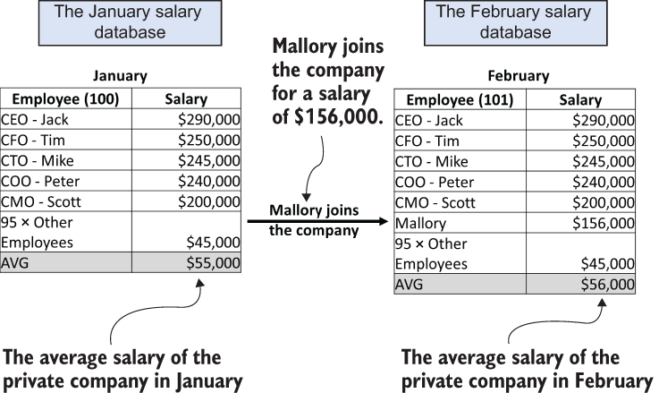
Figure 2.4 An excerpt from our private company’s database

Let’s start with the easier task, publishing the total number of employees. First, we’ll derive the sensitivity. As we’ve explained, it does not matter whether an employee is leaving or joining the company; the influence on the total number of employees is 1, so the sensitivity of this task is 1. Second, we need to design the random noise that will be added to the total number of employees before publishing it. As discussed previously, the amount of noise should be positively correlated to the sensitivity and negatively correlated to the privacy budget (since less privacy budget means stronger privacy protection, thus requiring more noise). The random noise should be proportional to △f/ϵ, where△f is the sensitivity and ϵ is the privacy budget.

In this example, we could draw our random noise from the zero-mean Laplace distribution, which is a “double-sided” exponential distribution, illustrated in figure 2.5.

Figure 2.5 The Laplace distribution

With that, we can calculate b = △f/ϵ and draw random noise from Lap (x|△f/ϵ) to be added to the total number of employees. Figure 2.6 illustrates the published total number of employees for January and February while applying different privacy budgets (i.e., ϵ). Based on the definition of DP, better privacy protection usually means the numbers of employees published in January and February are closer to each other with a higher probability. In other words, the results have a lower probability of revealing Mallory’s information to anyone seeing those two published values. The utility performance usually refers to the accuracy of the computations of certain aggregated data or statistics. In this case, it refers to the difference between the published perturbed value and its real value, with a lower difference meaning better utility performance. There is usually a tradeoff between privacy protection and utility performance for any data anonymization algorithm, including DP. For instance, as ϵ decreases, more noise will be added, and the difference between the two published values will be closer to each other, thus leading to stronger privacy protection. In contrast, specifying a larger value for ϵ could provide better utility but less privacy protection.

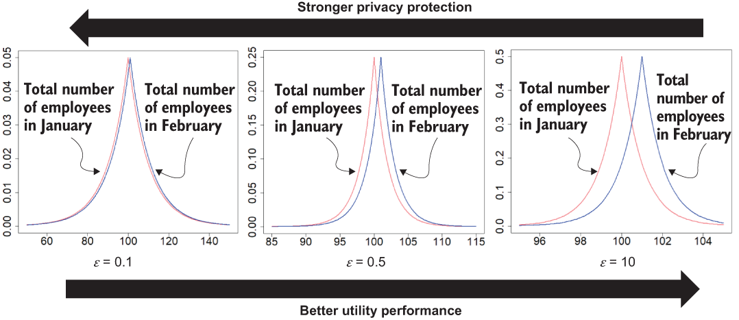
Figure 2.6 The tradeoff between privacy and utility

Now let’s consider the case of publishing the differentially private average salary. Regardless of whether any individual employee leaves or joins the company, the largest possible difference should come from the employee with the highest possible salary (in this case the CEO, Jack, who makes $290,000). For instance, in the extreme situation where there is only one employee in the database, and that happens to be the CEO, Jack, who has the highest possible salary, $290,000, his leaving would result in the largest possible difference to the company’s average salary. Hence, the sensitivity should be $290,000. We can now follow the same procedure as we did for the total number of employees, adding random noise drawn from Lap (x|△f/ϵ).

We’ll look at the details of applying random noise drawn from the Laplace distribution in the next section. For more information regarding the mathematics and formal definition of DP, refer to section A.1 of the appendix.

2.2 Mechanisms of differential privacy

In the last section we introduced the definition and usage of DP. In this section we’ll discuss some of the most popular mechanisms in DP, which will also become building blocks for many DP ML algorithms that we’ll introduce in this book. You can also use these mechanisms in your own design and development.

We’ll start with an old but simple DP mechanism—binary mechanism (randomized response).

2.2.1 Binary mechanism (randomized response)

Binary mechanism (randomized response) [5] is an approach that has long been utilized by social scientists in social science studies (since the 1970s), and it is much older than the formulation of DP. Although the randomized response is simple, it satisfies all the requirements of a DP mechanism.

Let’s assume that we need to survey of a group of 100 people on whether they have used marijuana in the last 6 months. The answer collected from each individual will be either yes or no, which is considered a binary response. We can give the value 1 to each “yes” answer and 0 to each “no” answer. Thus, we can obtain the percentage of marijuana usage in the survey group by counting the number of 1s.

To protect the privacy of each individual, we could apply a small amount of noise to each real answer before the submitted answer is collected. Of course, we are also hoping that the added noise will not alter the final survey results. To design a differentially private solution to collect the survey data, we could use a balanced coin (i.e., p = 0.5) for the randomized response mechanism, which proceeds as follows and is depicted in figure 2.7:

1. Flip a balanced coin.

2. If it comes up heads, the submitted answer is the same as the real answer (0 or 1).

3. If the coin comes up tails, flip the balanced coin one more time, and answer 1 if it comes up heads and 0 if tails.

Figure 2.7 How the binary mechanism (randomized response) works

The randomization in this algorithm comes from the two coin flips. This randomization creates uncertainty about the true answer, which provides the source of privacy. In this case, each data owner has a 3/4 probability of submitting the real answer and 1/4 chance of submitting the wrong answer. For a single data owner, their privacy will be preserved, since we will never be sure whether they are telling the truth. But the data user that conducts the survey will still get the desired answers, since 3/4 of the participants are expected to tell the truth.

Let’s revisit the definition of ϵ-DP (a more detailed and formal definition of DP can be found in section A.1). Let’s say we have a simple randomized response mechanism, which we’ll call M for now. This M satisfies ϵ-DP for every two neighboring databases or datasets, x, y, and for every subset S ⊆ Range(M),

In our example with the two coin flips, the data is either 1 or 0, and the output of M is also either 1 or 0. Hence, we have the following:

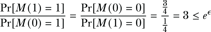
We can deduce that our simple randomized response mechanism M satisfies ln(3)-DP, where ln(3) is the privacy budget (ln(3) ≈ 1.099).

The basic idea of randomized response is that, while answering a binary question, one can tell the truth with higher probability and give the false answer with lower probability. The utility can be maintained by the somewhat higher probability of telling the truth, while privacy is theoretically protected by randomizing one’s response. In the previous example, we assumed that the coin is balanced. If we used an unbalanced coin, we could formulate a randomized response mechanism that satisfies other DP privacy budgets.

Based on the mechanism in figure 2.7, let’s assume the coin will come up heads with probability p and come up tails with probability (1 − p), where p > 1/2:

• Given an arbitrary survey participant, their answer will be either 0 or 1, depending on whether the participant answered truthfully with a “no” or “yes.”

• The output of our randomized response mechanism M can also be either 0 or 1.

Based on the definition of DP, we have

Then we have

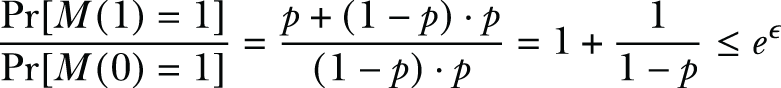
Since we assume p > 1/2, we have

Therefore, the privacy budget of using an unbalanced coin is

That is the general formulation for calculating the privacy budget for the randomized response mechanism.

Now let’s try to formulate the concept with pseudocode, where x indicates the true value, and it can be either 0 or 1:

def randomized_response_mechanism(x, p):
    if random() < p:
        return x
    elif random() < p:
        return 1
    else:
        return 0

Let’s take a closer look at the privacy budget of our binary mechanism while using different values for p (i.e., the probability of the coin coming up heads). Based on the preceding analysis, if p = 0.8, the privacy budget of our binary mechanism would be ln(1 + 0.8/(0.2 × 0.2)), leading to ln(21), which is 3.04. We can compare this to the earlier p = 0.5 example, whose privacy budget was ln(3) = 1.099.

As we discussed in the previous section, the privacy budget can be considered a measure of tolerance to privacy leakage. In this example, a higher p value means less noise is added (since it will generate the true answer with a higher probability), leading to more privacy leakage and a higher privacy budget. In essence, with this binary mechanism, the users can adjust the p value to accommodate their own privacy budget.

2.2.2 Laplace mechanism

In the binary mechanism, the privacy budget was determined by the probability of flipping a coin. In contrast, the Laplace mechanism achieves DP by adding random noise drawn from a Laplace distribution to the target queries or functions [6]. We already touched on the Laplace mechanism in the solution to our private company scenario. In this section we’ll introduce the Laplace mechanism in a more systematic way and walk through some examples.

Let’s go back to our private company scenario. To design a differentially private solution using the Laplace mechanism, we simply perturbed the output of the query function f (e.g., the total number of employees or the average salary) with random noise drawn from a Laplace distribution whose scale was correlated to the sensitivity of the query function f (divided by the privacy budget ϵ).

According to the design of the Laplace mechanism, given a query function f(x) that returns a numerical value, the following perturbed function satisfies ϵ-DP,

where △f is the sensitivity of query function f(x), and Lap (△f/ϵ) denotes the random noise drawn from the Laplace distribution with center 0 and scale △f/ϵ.

We established the concept of sensitivity in the previous section, but let’s do a refresh! Intuitively, the sensitivity of a function provides an upper bound on how much we have to perturb its output to preserve the individual’s privacy. For instance, in our previous example, where the database contains all employees’ salaries and the query function aims to calculate the average salary of all employees, the sensitivity of the query function should be determined by the highest salary in the database (e.g., the CEO’s salary). That’s because the higher the specific employee’s salary, the more influence it will have on the query’s output (i.e., the average salary) in the database. If we can protect the privacy of the employee with the highest salary, the privacy of the other employees is guaranteed. That’s why it is important to identify the sensitivity when designing a differentially private algorithm.

Now let’s explore some pseudocode that applies the Laplace mechanism:

def laplace_mechanism(data, f, sensitivity, epsilon):
    return f(data) + laplace(0, sensitivity/epsilon)

DP is typically designed and used in applications to answer specific queries. Before we go into any further detail, let’s explore some query examples that could apply the Laplace mechanism.

Example 1: Differentially private counting queries

Counting queries are queries of the form “How many elements in the database satisfy a given property P ?” Many problems can be considered counting queries. Let’s first consider a counting query regarding census data without applying DP.

In the following listing, we are calculating the number of individuals in the dataset who are more than 50 years old.

Listing 2.1 Counting query

import numpy as np
import matplotlib.pyplot as plt
ages_adult = np.loadtxt("https://archive.ics.uci.edu/ml/machine-learning-
➥ databases/adult/adult.data", usecols=0, delimiter=", ")

count = len([age for age in ages_adult if age > 50])      ❶
print(count)

❶ How many individuals in the census dataset are more than 50 years old?

The output will be 6,460.

Now let’s look at ways to apply DP to this kind of counting query. To apply DP on this query, we first need to determine the sensitivity of the query task, which is querying the number of individuals more than 50 years old. Since any single individual leaving or joining the census dataset could change the count at most by 1, the sensitivity of this counting query task is 1. Based on our previous description of the Laplace mechanism, we can add noise drawn from Lap(1/ϵ) to each counting query before publishing it, where ϵ is the privacy specified by the data owners. We can implement the DP version of this counting query by using NumPy’s random.laplace, as follows (using ϵ = 0.1, loc=0 for center 0):

sensitivity = 1
epsilon = 0.1

count = len([i for i in ages_adult if i > 50]) + np.random.laplace
➥ (loc=0, scale=sensitivity/epsilon)

print(count)

The output is 6,472.024,453,709,334. As you can see, the result of the differentially private counting query is still close to the real value of 6,460 while using ϵ= 0.1. Let’s try it with a much smaller ϵ(which means it will add more noise), ϵ= 0.001:

sensitivity = 1
epsilon = 0.001

count = len([i for i in ages_adult if i > 50]) + np.random.laplace
➥ (loc=0, scale=sensitivity/epsilon)

print(count)

The output is 7,142.911,556,855,243. As you can see, when we use ϵ = 0.001, the result has more noise added to the real value (6,460).

Example 2: Differentially private histogram queries

We can consider a histogram query to be a special case of a counting query, where the data is partitioned into disjoint cells and the query asks how many database elements lie in each of the cells. For example, suppose a data user would like to query the histogram of ages from the census data. How could we design a differentially private histogram query to study the distribution of ages without compromising the privacy of a single individual?

First, let’s first explore a histogram query of ages on the census data without DP.

Listing 2.2 Histogram query without DP

import numpy as np
import matplotlib.pyplot as plt

ages_adult = np.loadtxt("https://archive.ics.uci.edu/ml/machine-learning-
➥ databases/adult/adult.data",
                        usecols=0, delimiter=", ")
hist, bins = np.histogram(ages_adult)
hist = hist / hist.sum()

plt.bar(bins[:-1], hist, width=(bins[1]-bins[0]) * 0.9)
plt.show()

We will get output similar to figure 2.8.

Figure 2.8 Output of the histogram query without DP

To apply DP on this histogram query, we first need to calculate the sensitivity. Since the sensitivity of a histogram query is 1 (adding or deleting the information of a single individual can change the number of elements in a cell by at most 1), the sensitivity of the histogram query task is 1. Next, we need to add noise drawn from Lap (1/ϵ) to each of the histogram cells before publishing it, where ϵ is the privacy budget specified by the data owners.

We could easily implement the DP version of this histogram query using NumPy’s random.laplace, as in our previous example. Here we will explore an implementation using IBM’s Differential Privacy Library, diffprivlib.

First, install diffprivlib and import diffprivlib.mechanisms.Laplace:

!pip install diffprivlib
Laplace

Now we can implement the DP version of the histogram query using diffprivlib .mechanisms.Laplace.

Listing 2.3 DP version of the histogram query

def histogram_laplace(sample, epsilon=1, bins=10, range=None, normed=None,
➥  weights=None, density=None):
  hist, bin_edges = np.histogram(sample, bins=bins, range=range, 
  ➥ normed=None, weights=weights, density=None)
  dp_mech = Laplace(epsilon=1, sensitivity=1)
  dp_hist = np.zeros_like(hist)

  for i in np.arange(dp_hist.shape[0]):
    dp_hist[i] = dp_mech.randomise(int(hist[i]))

  if normed or density:
    bin_sizes = np.array(np.diff(bin_edges), float)
    return dp_hist / bin_sizes / dp_hist.sum(), bin_edges

  return dp_hist, bin_edges

Then the differentially private histogram query works as follows (ϵ = 0.01):

dp_hist, dp_bins = histogram_laplace(ages_adult, epsilon=0.01)
dp_hist = dp_hist / dp_hist.sum()

plt.bar(dp_bins[:-1], dp_hist, width=(dp_bins[1] - dp_bins[0]) * 0.9)
plt.show()

The output will look like the right side of figure 2.9. Can you see the difference between the histogram queries before and after applying DP? Even after applying DP, the shape of the distribution is still essentially the same, isn’t it?

Figure 2.9 Comparing the histogram queries before and after applying DP

The preceding two examples demonstrate that the most important step when applying the Laplace mechanism is to derive the appropriate sensitivity for a given application. Let’s go through some exercises to learn how to determine the sensitivity of the Laplace mechanism in different situations. 

Exercise 1: Differentially private frequency estimation

Suppose we have a class of students, some of whom like to play football, while others do not (see table 2.1). The teacher wants to know which of the two groups has the greatest number of students. This question can be considered a special case of the histogram query. What’s the sensitivity of this application?

Table 2.1 Students who do and don’t like football

Hint: Every student in the class can either like football or not, so the sensitivity is 1. Based on our description of the Laplace mechanism, we can simultaneously calculate the frequency of students who like football or not by adding noise drawn from Lap(1/ϵ) to each frequency, where ϵ is the privacy budget specified by the students. You may base your solution on the following pseudocode implementation:

sensitivity = 1
epsilon = 0.1

frequency[0] is the number of students who like football
frequency[1] is the number of students do not like football

dp_frequency = frequency[i] + np.random.laplace(loc=0,
➥ scale=sensitivity/epsilon)

Exercise 2: Most common medical condition for COVID-19

Suppose we wish to know which condition (among different symptoms) is approximately the most common for COVID-19 in the medical histories of a set of patients (table 2.2):

• What’s the sensitivity of this application?

• If we want to generate a histogram of the medical conditions for COVID-19, what should the sensitivity be?

Table 2.2 Symptoms of COVID-19 patients

Hints:

• Since individuals can experience many conditions, the sensitivity of this set of questions can be high. However, if we only report the most common medical condition, each individual at most results in a 1 number difference. Thus, the sensitivity of the most common medical condition is still 1. We could get the ϵ-differentially private result by adding noise drawn from Lap (1/ϵ) to each output of the most common medical condition.

• What if we want to generate a histogram of the medical conditions for COVID-19? What should the sensitivity be? Since each individual could experience multiple conditions (and at most could have all the conditions), the sensitivity is much more than 1—it could be the total number of different medical conditions reported for COVID-19. Therefore, the sensitivity of the histogram of the medical conditions for COVID-19 should equal to the total number of medical conditions, which is 7, as shown in table 2.2.

2.2.3 Exponential mechanism

The Laplace mechanism works well for most query functions that result in numerical outputs and where adding noise to the outputs will not destroy the overall utility of the query functions. However, in certain scenarios, where the output of a query function is categorical or discrete, or where directly adding noise to the outputs would result in meaningless outcomes, the Laplace mechanism runs out of its magical power.

For example, given a query function that returns the gender of a passenger (male or female, which is categorical data), adding noise drawn from the Laplace mechanism would produce meaningless results. There are many such examples, such as the value of a bid in an auction [4], where the purpose is to optimize revenue. Even though the auction prices are real values, adding even a small amount of positive noise to the price (to protect the privacy of a bid) could destroy an evaluation of the resulting revenue.

The exponential mechanism [7] was designed for scenarios where the goal is to select the “best” response but where adding noise directly to the output of the query function would destroy the utility. As such, the exponential mechanism is the natural solution for selecting one element from a set (numerical or categorical) using DP.

Let’s see how we can use the exponential mechanism to provide ϵ-DP for a query function f. Here are the steps:

1. The analyst should define a set A of all possible outputs of the query function f.

2. The analyst should design a utility function (a.k.a. a score function) H, whose input is data x and the potential output of f(x), denoted as a ∈ A. The output of H is a real number. △H denotes the sensitivity of H.

3. Given data x, the exponential mechanism outputs the element a ∈ A with probability proportional to exp(ϵ ⋅H(x, a)/(2ΔH)).

Let’s explore some examples that could apply the exponential mechanism, so you can see how to define the utility functions and derive the sensitivities.

Example 3: Differentially private most common marital status

Suppose a data user wants to know the most common marital status in the census dataset. If you load the dataset and quickly go through the “marital-status” column, you will notice that the records include seven different categories (married-civ-spouse, divorced, never-married, separated, widowed, married-spouse-absent, married-AF-spouse).

Let’s first take a look at the number of people in each category in the dataset. Before proceeding with listing 2.4, you will need to download the adult.csv file from the book’s code repository found at https://github.com/nogrady/PPML/.

Listing 2.4 Number of people in each marital status group

import matplotlib.pyplot as plt
import pandas as pd
import numpy as np

adult = pd.read_csv("adult.csv")

print("Married-civ-spouse: "+ str(len([i for i in adult['marital-status']
➥ if i == 'Married-civ-spouse'])))
print("Never-married: "+ str(len([i for i in adult['marital-status']
➥ if i == 'Never-married'])))
print("Divorced: "+ str(len([i for i in adult['marital-status']
➥ if i == 'Divorced'])))
print("Separated: "+ str(len([i for i in adult['marital-status']
➥ if i == 'Separated'])))
print("Widowed: "+ str(len([i for i in adult['marital-status']
➥ if i == 'Widowed'])))
print("Married-spouse-absent: "+ str(len([i for i in adult['marital-
➥ status'] if i == 'Married-spouse-absent'])))
print("Married-AF-spouse: "+ str(len([i for i in adult['marital-status']
➥ if i == 'Married-AF-spouse'])))

The result will look like the following:

Married-civ-spouse: 22379
Never-married: 16117
Divorced: 6633
Separated: 1530
Widowed: 1518
Married-spouse-absent: 628
Married-AF-spouse: 37

As you can see, Married-civ-spouse is the most common marital status in this census dataset.

To use the exponential mechanism, we first need to design the utility function. We could design it as H(x, a), which is proportional to the number of people of each marital status x, where x is one of the seven marital categories and a is the most common marital status. Thus, a marital status that includes a greater number of people should have better utility. We could implement this utility function as shown in the following code snippet:

adult = pd.read_csv("adult.csv")
sets = adult['marital-status'].unique()

def utility(data, sets):
    return data.value_counts()[sets]/1000

With that, we can move into designing a differentially private most common marital status query function using the exponential mechanism.

Listing 2.5 Number of people in each marital status group, with exponential mechanism

def most_common_marital_exponential(x, A, H, sensitivity, epsilon):
    utilities = [H(x, a) for a in A]                                     ❶
    
    probabilities = [np.exp(epsilon * utility / (2 * sensitivity))
    ➥ for utility in utilities]                                         ❷
    
    probabilities = probabilities / np.linalg.norm(probabilities, ord=1) ❸


    return np.random.choice(A, 1, p=probabilities)[0]                    ❹

❶ Calculate the utility for each element of A.

❷ Calculate the probability for each element, based on its utility.

❸ Normalize the probabilities so they sum to 1.

❹ Choose an element from A based on the probabilities.

Before using this query, we need to determine the sensitivity and the privacy budget. For the sensitivity, since adding or deleting the information of a single individual can change the utility score of any marital status by at most 1, the sensitivity should be 1. For the privacy budget, let’s try ϵ = 1.0 first:

most_common_marital_exponential(adult['marital-status'], sets,
➥ utility, 1, 1)

As you can see, the output is Married-civ-spouse. To better illustrate the performance of most_common_marital_exponential, let’s check the result after querying it 10,000 times:

res = [most_common_marital_exponential(adult['marital-status'], sets,
➥ utility, 1, 1) for i in range(10000)]
pd.Series(res).value_counts()

You will get output similar to the following:

Married-civ-spouse       9545
Never-married             450
Divorced                    4
Married-spouse-absent       1

According to these results, most_common_marital_exponential could randomize the output of the most common marital status to provide privacy protection. However, it also produces the actual result (Married-civ-spouse) with the highest probability of providing utility.

You can also check these results by using different privacy budgets. You’ll observe that with a higher privacy budget, it is more likely to result in Married-civ-spouse, which is the true answer.

Exercise 3: Differentially private choice from a finite set

Suppose the people in a city want to vote to decide what kind of sports competition they want in the summer. Since the city’s budget is limited, only one competition from four choices (football, volleyball, basketball, and swimming) is possible, as shown in table 2.3. The mayor wants to make the voting differentially private, and each person has one vote. How can we publish the voting results in a differentially private way by using the exponential mechanism?

Table 2.3 Votes for different sports

Hint: To use the exponential mechanism, we should first decide on the utility function. We could design the utility function as H(x, a), which is proportional to the number of votes for each category x, where x is one of the four sports, and a is the sport that has the highest vote. Thus, the sport that has a higher number of votes should have better utility. Then we could apply the exponential mechanism to the voting results to achieve ϵ-DP.

The pseudocode for the utility function could be defined as follows:

def utility(data, sets):
    return data.get(sets)

We can then implement the differentially private votes query function using the exponential mechanism with the following pseudocode.

Listing 2.6 Differentially private votes query

def votes_exponential(x, A, H, sensitivity, epsilon):
    utilities = [H(x, a) for a in A]                                      ❶
    
    probabilities = [np.exp(epsilon * utility / (2 * sensitivity))
    ➥ for utility in utilities]                                          ❷
    
    probabilities = probabilities / np.linalg.norm(probabilities, ord=1)  ❸

    return np.random.choice(A, 1, p=probabilities)[0]                     ❹

❶ Calculate the utility for each element of A.

❷ Calculate the probability for each element, based on its utility.

❸ Normalize the probabilities so they sum to 1.

❹ Choose an element from A based on the probabilities.

As with any mechanism, we need to determine the sensitivity and the privacy budget before using this query. For the sensitivity, since each voter can only vote for one type of sport, each individual can change the utility score of any sport by at most 1. Hence, the sensitivity should be 1. For the privacy budget, let’s try ϵ = 1.0 first.

We could call the DP query function as shown in the following pseudocode:

A = ['Football', 'Volleyball', 'Basketball', 'Swimming']
X = {'Football': 49, 'Volleyball': 25, 'Basketball': 6, 'Swimming':2}
votes_exponential(X, A, utility, 1, 1)

Given this implementation, your results should be similar to example 3, with it outputting football (the sport with the highest votes) with a higher probability. When you use a higher privacy budget, it will be more likely to select football correctly.

In this section we’ve introduced the three most popular mechanisms in DP in use today, and they are the building blocks for many differentially private ML algorithms. Section A.2 of the appendix lists some more advanced mechanisms that can be utilized in special scenarios, some of which are variations on the Laplace and exponential mechanisms.

So far, with our private company example, we’ve designed solutions for tasks (the total number of employees, and the average salary) that will satisfy DP individually. However, these tasks are not independent of each other. Conducting both tasks at the same time (sharing both the total number of employees and the average salary) requires further analysis in terms of the DP properties. That’s what we’ll do next.

2.3 Properties of differential privacy

Thus far, you have learned the definition of DP and seen how to design a differentially private solution for a simple scenario. DP also has many valuable properties that make it a flexible and complete framework for enabling privacy-preserving data analysis on sensitive personal information. In this section we’ll introduce three of the most important and commonly utilized properties for applying DP.

2.3.1 Postprocessing property of differential privacy

In most data analysis and ML tasks, it takes several processing steps (data collection, preprocessing, data compression, data analysis, etc.) to accomplish the whole task. When we want our data analysis and ML tasks to be differentially private, we can design our solutions within any of the processing steps. The steps that come after applying the DP mechanisms are called postprocessing steps.

Figure 2.10 illustrates a typical differentially private data analysis and ML scenario. First, the private data (D₁) is stored in a secure database controlled by the data owner. Before publishing any information (such as a sum, count, or model) regarding the private data, the data owner will apply the DP sanitizer (DP mechanisms that add random noise) to produce the differentially private data (D₂). The data owner could directly publish D₂ or conduct postprocessing steps to get D₃ and publish D₃ to the data user.

Figure 2.10 Postprocessing property of differential privacy

It is noteworthy that the postprocessing steps could actually reduce the amount of random noise added by the DP sanitizer to the private data. Let’s continue to use our private company scenario as a concrete example.

As you saw earlier, the private company designed a differentially private solution for publishing its total number of employees and average salary by adding random noise drawn from Laplace distributions scaled to △f/ϵ, where △f is the sensitivity and ϵ is the privacy budget. This solution perfectly satisfies the concept of DP. However, directly publishing the data after adding the random noise could lead to potential problems, since the noise drawn from the zero-mean Laplace distribution is a real number and could also be negative real numbers (with 50% probabilities). For instance, adding Laplace random noise to the total number of employees could result in non-integer numbers, such as 100 −> 100.5 (+0.5 noise), and negative numbers, such as 5 −> −1 (−6 noise), which is meaningless.

A simple and natural solution to this problem involves postprocessing by rounding negative values up to zero, and values that are larger than n can be rounded down to n (the next integer): 100.5 −> 100 (round down real value to the next integer), −1 −> 0 (round up negative value to zero).

As you can see, this postprocessing step solves the problem, but it could also reduce the amount of noise added to the private data as compared to when postprocessing was not being done. For instance, suppose y is the private data and ȳ is the perturbed data, where ȳ = y + Lap(Δf/ϵ), and y' is the rounded up perturbed data. If y is positive due to the addition of Laplacian noise, ȳ is negative. By rounding ȳ up to zero (i.e., ŷ' = 0), we can clearly see that it becomes closer to the true answer so that the amount of noise added has been reduced. The same conclusion could also be reached for the case where ȳ is a real number but greater than y.

At this point, a question could be raised: will this solution remain differentially private even after we perform the previously described postprocessing step? The short answer is yes. DP is immune to postprocessing [3], [4]. The postprocessing property guarantees that given the output of a differentially private algorithm (one that satisfies ϵ-DP), any other data analyst, without additional knowledge about the original private database or dataset, cannot come up with any postprocessing mechanism or algorithm to make the output less differentially private. To summarize: If an algorithm M(x) satisfies ϵ-DP, then for any (deterministic or randomized) function F(⋅), F(M(x)) satisfies ϵ-DP.

Based on the postprocessing property of DP, once the sensitive data of an individual is claimed to be protected by a randomized algorithm, no other data analyst can increase its privacy loss. We can consider postprocessing techniques to be any de-noising, aggregation, data analysis, and even ML operations on the DP private data that do not directly involve the original private data.

2.3.2 Group privacy property of differential privacy

In our previous examples, we only discussed privacy protection or leakage for a single individual. Let’s now look at an example of privacy protection or leakage that could involve a group of people.

Figure 2.11 shows a scenario where there are k scientists who collaboratively conduct a research study by sharing their results with each other. A real-world example would be the case of different cancer research institutions collaboratively working on a research study to discover a new drug. They cannot share patients’ records or the formula due to privacy concerns, but they can share the sanitized results.

Figure 2.11 The group privacy property of differential privacy

Now assume that news reporter Alice would like to report on the study’s highlights without revealing the secrets of the study by interviewing each of the k scientists. To ensure none of the scientists reveal secrets about their research study, the scientists designed a protocol to follow while each of them is interviewed by the reporter, such that whatever information is exchanged about the research study should be sanitized by an ϵ-DP randomized mechanism.

Alice conducted the interviews with each of the k scientists and published her report. However, more recently, it was found that Eve, a competitor scientist, learned the details about the research study beyond what was exchanged with Alice just based on Alice’s report. What could have happened?

Recall from the definition of DP that ϵ is the privacy budget that controls how much the output of a randomized mechanism can differ from the real-world scenario. It can be shown that the difference between the output of the ϵ-differentially private randomized mechanism from the k scientists and the real-world scenario grows to at most a privacy budget of k ⋅ ϵ. Therefore, even though interviewing each scientist only cost a privacy budget of ϵ, since the k scientists share the same secret, interviewing all of them actually costs a privacy budget of k ⋅ ϵ. As such, the privacy guarantee degrades moderately as the size of the group increases. If k is large enough, Eve could learn everything about the research study, even though each of the k scientists follows an ϵ-differentially private randomized mechanism when answering during the interviews. A meaningful privacy guarantee can be provided to groups of individuals up to a size of about k ≈ 1/ϵ. However, almost no protection is guaranteed to groups of k ≈ 100/ ϵ.

The k scientists example illustrates the group property of DP, where sometimes a group of members (such as families or employees of a company) would like to join an analytical study together, and the sensitive data might therefore have something to do with all the group members. To summarize: If algorithm M(x) satisfies ϵ-DP, applying M(x) to a group of k correlated individuals satisfies k ⋅ ϵ-DP.

The group privacy property of DP enables researchers and developers to design efficient and useful DP algorithms for a group of individuals. For instance, consider a scenario of federated learning (i.e., collaborative learning). In general, federated learning enables decentralized data owners to collaboratively learn a shared model while keeping all the training data local. In essence, the idea is to perform ML without the need to share training data. At this point, it is important to protect the privacy of each data owner who owns a group of data samples, but not each sample itself, where DP can play a big role.

2.3.3 Composition properties of differential privacy

Another very important and useful property of DP is its composition theorems. The rigorous mathematical design of DP enables the analysis and control of cumulative privacy loss over multiple differentially private computations. Understanding these composition properties will enable you to better design and analyze more complex DP algorithms based on simpler building blocks. There are two main composition properties, and we’ll explore them next.

Sequential composition

In data analysis and ML, the same information (statistics, aggregated data, ML models, etc.) is usually queried multiple times. For instance, in our previous private company scenario, the total number of employees and the average salary could be queried by different people (such as Alice and Bob) multiple times. Even though random noise is added to the queried results each time, more queries will cost more privacy budget and potentially result in more privacy leakage. For instance, if Alice or Bob could gather enough noisy query results from the current (static) database, they could cancel the noise simply by calculating the average of those noisy query results, since the random noise is always drawn from the same zero mean Laplace distribution. Therefore, we should be careful when designing a differentially private solution for private data that requires multiple sequential queries.

To illustrate the sequential composition property of DP, let’s consider another scenario. Suppose Mallory’s personal information (her salary) is contained in the private company’s employee information database that is used by a potential business analyzer in two separate differentially private queries. The first query might be about the average salary of the company, while the second query might be about the number of people who have a salary higher than $50,000. Mallory is concerned about these two queries, because when the two results are compared (or combined), they could reveal the salaries of individuals.

The sequential composition property of DP confirms that the cumulative privacy leakage from multiple queries on data is always higher than the single query leakage. For example, if the first query’s DP analysis is performed with a privacy budget of ϵ₁ = 0.1, and the second has a privacy budget of ϵ₂ = 0.2, the two analyses can be viewed as a single analysis with a privacy loss parameter that is potentially larger than ϵ₁ or ϵ₂ but at most ϵ₃ = ϵ₁ + ϵ₂ = 0.3. To summarize: If algorithm F₁(x) satisfies ϵ₁-DP, and F₂(x) satisfies ϵ₂-DP, the sequential composition of F₁(x) and F₂(x) satisfies (ϵ₁ + ϵ₂)-DP.

Now let’s explore an example that demonstrates the sequential composition property of DP.

Example 4: Sequential composition of differentially private counting queries

Let’s reconsider the scenario shown in example 1, where we wanted to determine how many individuals in the census dataset were more than 50 years old. The difference is that now we have two DP functions with different privacy budgets. Let’s see what will happen after applying different DP functions sequentially.

In the following listing, we define four DP functions, where F₁ satisfies 0.1-DP (ϵ₁ = 0.1), F₂ satisfies 0.2-DP (ϵ₂ = 0.2), F₃ satisfies 0.3-DP (ϵ₃ = ϵ₁ + ϵ₂), and F_seq is the sequential composition of F₁ and F₂.

Listing 2.7 Applying sequential composition

import numpy as np
import matplotlib.pyplot as plt
ages_adult = np.loadtxt("https://archive.ics.uci.edu/ml/machine-learning-
➥ databases/adult/adult.data", usecols=0, delimiter=", ")
 
sensitivity = 1
epsilon1 = 0.1
epsilon2 = 0.2
epsilon3 = epsilon1 + epsilon2
 
def F1(x):                                                            ❶
    return x+np.random.laplace(loc=0, scale=sensitivity/epsilon1)     ❶
 
def F2(x):                                                            ❷
    return x+np.random.laplace(loc=0, scale=sensitivity/epsilon2)     ❷
 
def F3(x):                                                            ❸
    return x+np.random.laplace(loc=0, scale=sensitivity/epsilon3)     ❸
 
def F_seq(x):                                                         ❹
    return (F1(x)+F2(x))/2                                            ❹

❶ Satisfies 0.1-DP

❷ Satisfies 0.2-DP

❸ Satisfies 0.3-DP

❹ The sequential composition of F1 and F2

Now, given that x is the real value of “how many individuals in the census dataset are more than 50 years old?” let’s compare the output of F₁, F₂, and F₃:

x = len([i for i in ages_adult if i > 50])
 
plt.hist([F1(x) for i in range(1000)], bins=50, label='F1');            ❶
 
plt.hist([F2(x) for i in range(1000)], bins=50, alpha=.7, label='F2');  ❷
 
plt.hist([F3(x) for i in range(1000)], bins=50, alpha=.7, label='F3');  ❸
 
plt.legend();

❶ Plot F1

❷ Plot F2 (should look the same)

❸ Plot F3 (should look the same)

In figure 2.12 you can see that the distribution of outputs from F₃ looks “sharper” than that of F₁ and F₂ because F₃ has a higher privacy budget (ϵ) that indicates more privacy leakage and thus a higher probability of outputting results close to the true answer (6,460).

Figure 2.12 Output of sequential composition of differentially private counting queries

Now let’s compare the output of F₃ and F_seq, as shown in the following code snippet:

plt.hist([F_seq(x) for i in range(1000)], bins=50, alpha=.7,
➥ label='F_seq');                                                       ❶
 
plt.hist([F3(x) for i in range(1000)], bins=50, alpha=.7, label='F3');   ❷
 
plt.legend();

❶ Plot F_seq

❷ Plot F3

As you can see in figure 2.13, the output of F₃ and F_seq are about the same, which demonstrates the sequential composition property of DP. But it is noteworthy that the sequential composition only defines an upper bound on the total ϵ of the sequential composition of several DP functions (i.e., the worst-case privacy leakage). The actual cumulative effect on the privacy might be lower. For more information regarding the mathematical theory of the sequential composition of DP, see section A.3.

Figure 2.13 Comparing the distribution of outputs F₃ and F_seq

Parallel composition

At this point, an obvious question is what will happen if someone combines several different DP algorithms in parallel. To illustrate the parallel composition property of DP, consider the following scenario.

Suppose company A maintains a database of its employees’ salary information. Alice wants to learn the number of employees at company A whose salaries are higher than $150,000, while Bob would like to study the number of employees at company A whose salaries are less than $20,000. To meet the company’s privacy protection requirements, Alice is asked to use ϵ₁-DP mechanisms to access the database, while Bob is required to apply ϵ₂-DP mechanisms to get the information from the same database. What’s the total privacy leakage from Alice’s and Bob’s access to the database?

Since the employees whose salaries are higher than $150,000 and the employees whose salaries are less than $20,000 are two disjoint sets of individuals, releasing both sets of information will not cause any privacy leakage for the same employee twice. For instance, if ϵ₁ = 0.1 and ϵ₂ = 0.2, per the parallel composition property of DP, Alice’s and Bob’s accesses to the database utilize a total of ϵ₃ = max(ϵ₁, ϵ₂) = 0.2 privacy budget.

To summarize: If algorithm F₁(x₁) satisfies ϵ₁-DP, and F₂(x₂) satisfies ϵ₂-DP, where (x₁, x₂) is a nonoverlapping partition of the whole dataset x, the parallel composition of F₁(x₁) and F₂(x₂) satisfies max(ϵ₁,ϵ₂)-DP. max(ϵ₁,ϵ₂) defines an upper bound on the total ϵ of parallel composition of several DP functions (i.e., the worst-case privacy leakage); the actual cumulative effect on the privacy might be lower. For more information regarding the mathematical theory behind parallel composition of DP, see section A.4.

The sequential and parallel composition properties of DP are considered inherent properties of DP, where the data aggregator does not need to make any special effort to calculate the privacy bound while composing multiple DP algorithms. Such composition properties of DP enable researchers and developers to focus more on the design of simpler differentially private building blocks (i.e., mechanisms), and a combination of those simpler building blocks can be used directly to solve much more complex problems.

Summary

• DP is a promising and popular privacy-enhancing technique that provides a rigorous definition of privacy.

• DP aims to strengthen privacy protection by releasing the aggregated or statistical information of a database or dataset without revealing the presence of any individual in that database.

• The sensitivity usually measures the maximum possible effect of each individual’s information on the output of the analysis.

• The privacy budget ϵ is usually set by the data owners to tune the level of privacy protection required.

• DP can be implemented by perturbing the aggregation or statistics of the sensitive information using different DP mechanisms.

• In the binary mechanism, randomization comes from the binary response (the coin flip), which helps to perturb the results.

• The Laplace mechanism achieves DP by adding random noise drawn from a Laplace distribution to the target queries or functions.

• The exponential mechanism helps cater for scenarios where the utility is to select the best response but where adding noise directly to the output of the query function would fully destroy the utility.

• DP is immune to postprocessing: once the sensitive data of an individual’s DP is claimed to be protected by a randomized algorithm, no other data analyst can increase its privacy loss without involving information about the original sensitive data.

• DP can be applied to analyze and control the privacy loss coming from groups, such as families and organizations.

• DP also has sequential and parallel composition properties that enable the design and analysis of complex differentially private algorithms from simpler differentially private building blocks.