6 Privacy-preserving synthetic data generation

This chapter covers

• Synthetic data generation
• Generating synthetic data for anonymization
• Using differential privacy mechanisms to generate privacy-preserving synthetic data
• Designing a privacy-preserving synthetic data generation scheme for machine learning tasks

So far we’ve looked into the concepts of differential privacy (including the centralized, DP, and the local, LDP, versions) and their applications in developing privacy-preserving query-processing and machine learning (ML) algorithms. As you saw, the idea of DP is to add noise to the query results (without disturbing their original properties) such that the results can assure the privacy of the individuals while satisfying the utility of the application.

But sometimes data users may request the original data to utilize it locally and directly, perhaps to develop new queries and analysis procedures. Privacy-preserving data-sharing methods can be used for such purposes. This chapter will look into synthetic data generation—a promising solution for data sharing—which generates synthetic yet representative data that can be shared among multiple parties safely and securely. The idea of synthetic data generation is to artificially generate data that has distribution and properties similar to the original data. And because it is artificially produced, we do not have to worry about privacy concerns.

We’ll start this chapter by introducing the concepts and basics of synthetic data generation. Subsequent sections will present implementations of synthetic data generation approaches using different data anonymization techniques or DP. Toward the end of this chapter, we’ll walk you through a case study that implements a novel privacy- preserving synthetic data generation approach using data anonymization and DP for ML purposes.

6.1 Overview of synthetic data generation

In essence, data is a collection of facts that can be translated into a form that a computer can understand and process. With today’s modern applications, data collection happens almost everywhere, such as in business analytics, engineering optimization, social science analysis, scientific research, and so on. Typically, different characteristics or patterns of data can be used to achieve various objectives. For instance, in healthcare applications, diverse image data such as x-rays, CT scans, and dermoscopic images can be used by ML applications to diagnose particular diseases or aid treatments.

However, in practice, it is very challenging to obtain real (and sensitive) data for many reasons, including privacy concerns, and even when you can collect the data, you are usually not permitted to share it with other parties. When it comes to ML applications, most algorithms require a large amount of training data to achieve their best performance, but it is not always feasible to collect such an amount of real data. Thus, there is a need for synthetic (yet representative) data, and due to the aforementioned concerns, synthetic data has become an increasingly important and popular topic.

6.1.1 What is synthetic data? Why is it important?

The performance of an ML model largely depends on the amount and quality of data accumulated to train the model. When an organization does not have sufficient data for the training, data sharing often happens between organizations that have similar research interests. This enables the research to scale, but the privacy problem remains the same. The data usually includes sensitive personal information that can cause privacy leakage for the individuals. Hence, it is imperative to enable privacy-preserving mechanisms when data sharing. To that end, generating privacy-preserving synthetic data is one of the best alternatives—it is a flexible and viable next-step solution for sharing sensitive data across multiple stakeholders.

Synthetic data is a kind of artificially formulated data, usually generated with artificial algorithms rather than being collected by real-world direct measurement techniques. But it still carries some critical features of the actual data (e.g., statistical properties, functionalities, or conclusions). Analyzing the synthetic data can produce results similar to analyzing the actual data itself. Another advantage of synthetic data is that it can be generated for the specific characteristics of rare testing scenarios that are extremely hard to observe in reality (i.e., scenarios where it is challenging to obtain actual data). This enables the engineers and researchers to generate different datasets to validate various models, evaluate ML algorithms, and test new products, pipelines, and tools under different scenarios.

Moreover, synthetic data helps us ensure privacy protection. Synthetic data can have statistical characteristics similar to the original data without disclosing the original data, which paves a safer way of protecting privacy and confidentiality. For instance, primary care providers (such as hospitals) collect and share their patients’ information for research purposes with the consent of those patients. However, most patients will not agree to share their private information with other parties. Instead of sharing the original data, we can generate artificial or synthetic data based on the properties of the original dataset. Then we can share the synthetically produced data with other data users. That retains the utility of the application and preserves the privacy of the original data.

6.1.2 Application aspects of using synthetic data for privacy preservation

Synthetic data does not contain any personal information; it is an artificially produced dataset with a distribution similar to the original data. Hence, engineering, business, and scientific research applications can benefit from using synthetic data for privacy-preserving purposes.

For instance, let’s consider an example of sharing clinical and medical data between different healthcare entities (e.g., hospitals and research institutions). Let’s assume that two hospitals, A and B, plan to conduct a research program to learn the relationship between an individual’s specific personal information (age, BMI, glucose, etc.) and their probability of getting breast cancer. Both hospitals can collect valuable data from their patients, but because of the patient-hospital agreements, the two hospitals cannot share their data with each other. Furthermore, because the number of samples is limited, one hospital’s data is not sufficient to support such research. Hence, the two hospitals have to work together to conduct the research without compromising their patients’ personal information.

In this situation, we can use synthetic data generation techniques to produce synthetic yet representative data that can be safely shared. Typically, the generated synthetic data has the same format, statistics, and distribution as the original data (as shown in figure 6.1), without leaking any information from a single individual. Sharing a synthetic dataset in the same form as the original data gives much more flexibility in how data users can use it with no privacy concerns.

Figure 6.1 The synthetic data retains the structure of the original data, but they are not the same.

Synthetic data can also be utilized in business scenarios. For instance, suppose a company wants to conduct a business analysis to improve its marketing spend. To conduct this analysis, the company’s marketing units are usually required to have their customers’ consent to use their data. However, customers will likely not consent to share their data, since the data might contain sensitive information, such as transactions, locations, and shopping information. In this scenario, using synthetic data generated from the customers’ data will enable the company to run an accurate simulation for the business analysis without requiring the consent of the customers. Since the synthetic data is generated based on the statistical properties of the actual data, it can be reliably used in such studies.

6.1.3 Generating synthetic data

Before we look at specific generation techniques, let’s go through the general process of generating synthetic data, illustrated in figure 6.2.

Figure 6.2 General pipeline for generating synthetic data

Before extracting any statistical characteristics from the original dataset, the first step is to preprocess the original dataset by removing the outliers and normalizing the feature values. Outliers are data points distant from other observations. They may result from variability and measurement error in the experiments, which sometimes provide incorrect information to data users. In most cases, outliers are likely to mislead the synthetic data generator to generate more outliers, making the ML model inaccurate. One common way of detecting outliers is using a density-based method: observing if the probability of the presence of specific points in a certain area is much lower than the expected value in that area.

The next step is feature normalization. Each dataset has a different number of features, and each feature has a different range of values. Feature normalization usually scales all the features to the same range, which helps us extract the statistical characteristics while giving equal consideration to the different features. After normalizing the dataset, we can build the distribution extraction model, which keeps the statistical characteristics of the original data.

Finally, the privacy test is designed to ensure that the generated synthetic data satisfies certain predefined privacy guarantees (k-anonymity, DP, etc.). If the generated synthetic data cannot provide the predefined privacy guarantees, the privacy test will be failed. We can generate synthetic datasets repeatedly until one passes the privacy test.

Now that we have covered the basic concepts, the application scenarios, and the general synthetic data generation process, let’s look into some of the most popular synthetic generation techniques based on data anonymization and DP. We’ll start with the data anonymization approaches.

6.2 Assuring privacy via data anonymization

The previous chapters discussed different techniques for privatizing sensitive information by adding noise and using perturbation techniques. And as we discussed at the beginning of this chapter, synthetic data is artificially produced data. Hence, different data anonymization techniques can also be used to create a synthetic dataset.

In this section we’ll discuss historical non-DP approaches that use data anonymization techniques to share private and sensitive information without betraying the individual’s privacy. In section 6.3 we’ll discuss using DP for synthetic data generation.

6.2.1 Private information sharing vs. privacy concerns

Before we look at how anonymization techniques work, let’s consider the scenario where individuals’ medical records are released to the public for research purposes. Sharing such information has many benefits for research, including assisting the research community in confirming published results and facilitating them to do more qualitative in-depth analyses of the data. Thus, anonymizing the data is common before releasing data to the public.

But can we anonymize a dataset arbitrarily? In 1997, the Group Insurance Commission from Massachusetts wanted to release a dataset of hospital visits by state employees, which was to be used for research purposes [1]. Of course, there were privacy considerations, so they removed all the columns that could be used to identify who the patient was, such as name, phone number, SSN, and address. Do you think this data release went well?

Unfortunately, it did not. A researcher from MIT, Latanya Sweeney [2], found that even though the main identifiers were removed, some demographic information was left in the dataset, such as zip code, date of birth, and gender. Sweeney realized that the claims of the Massachusetts governor, who insisted that the privacy of the individuals was respected, were actually not correct. She decided to re-identify which records of the published (or anonymized) dataset were the governor’s, so she investigated the public voter records from Massachusetts, which had full identifiers, such as name, address, and demographic data, including zip code and date of birth. She was able to identify records of prescriptions and visits in the dataset that belonged to the governor.

Note In data security, a re-identification attack is when someone tries to link external data sources to identify a particular individual or a sensitive record.

As you can see, data anonymization techniques can be used to synthesize a dataset, but we need to make sure sensitive values in the dataset are no longer unique. How can we create an anonymized dataset such that none of the sensitive values in the dataset are unique? Here comes k-anonymity, a popular data anonymization approach.

6.2.2 Using k-anonymity against re-identification attacks

K-anonymity is a key security concept used to alleviate the risk of someone re-identifying anonymized data by linking it to external datasets [3]. The idea is simple. It uses techniques called generalization and suppression to hide an individual’s identity in a group of similar people. In technical terms, a dataset is said to be k-anonymous when every possible combination of values for sensitive columns appears at least for k different records, where k represents the number of records in that group. If, for any individual in a particular dataset, there are at least k-1 other individuals who have the same properties, we can say that dataset is k-anonymized.

For example, suppose we have the same Group Insurance Commission dataset, we are looking at the zip code in that dataset, and we set k to 20. If we look at any person in that dataset, we should always find 19 other individuals who share the same zip code. The bottom line is that we will not be able to specifically identify an individual just by referring to their zip code. The same concept can be extended further to combining multiple attributes. For example, we could consider both zip code and age as the attributes. In that case, the anonymized dataset should always have 19 other individuals sharing the same age and zip code, which makes re-identification much harder than in the previous case.

The dataset in table 6.1 is 2-anonymous, where every combination of values (in this case, zip code and age) appears at least k = 2 times.

Table 6.1 An example 2-anonymous dataset where every combination of zip code and age appears at least twice

How to make a synthetic dataset k-anonymous

There are two different techniques that can be used to make an original dataset k-anonymous: generalization and suppression.

In generalization, the main idea is to make a value less precise so that records with different values are generalized into records that share the same values. Let’s consider the original dataset shown in table 6.2 and the 2-anonymous version shown in table 6.3.

Table 6.2 The original dataset

Table 6.3 The 2-anonymous version of the dataset in table 6.2

Suppose table 6.2 represents the original dataset we are interested in, and we need to transform it to its 2-anonymous version. In this case, we can transform the numerical values in the dataset into numerical ranges so that the resulting table verifies 2-anonymity, as shown in table 6.3.

As you can see, even after the anonymization process, the resultant values are still relatively close to the original values in the dataset. For example, age 24 became the range of 20 to 29, but it is still close to the original.

Now let’s consider table 6.4. Here the first four records can simply be converted to their 2-anonymous versions. But the last record is an outlier. If we try to group it with one of the pairs, the result would have a very large range of values. For instance, age would range from 10 to 49, while the zip code would be completely removed. Hence, the simplest solution is to remove the outlier from the dataset and keep the rest of the records. That process is called suppression.

Table 6.4 An example dataset with an outlier. As you can see, age 12 in the last row is an outlier.

At a high level, this is how we can apply k-anonymity for a dataset to produce an anonymized (or synthetic) dataset. We will be discussing more detailed examples and techniques in chapter 7, along with hands-on exercises.

As you can see, by generalizing and suppressing the data, k-anonymity makes privacy leakage difficult. However, it has some drawbacks, which we will discuss next.

6.2.3 Anonymization beyond k-anonymity

While k-anonymity makes it harder to re-identify records, it also has some drawbacks. For example, suppose all individuals in a dataset share the same value for the attributes in consideration. In such a case, that information may be revealed simply by knowing that these individuals are part of the dataset.

Let’s consider the dataset in table 6.5. As you can see, it is already 2-anonymized, but what if Bob lives in the 33620 zip code and knows that his neighbor recently went for a medical appointment? Bob might deduce that his neighbor has heart disease. Therefore, even though Bob cannot distinguish which record belongs to his neighbor (thanks to k-anonymity), he can still infer which disease his neighbor has.

Table 6.5 Even with a k-anonymized dataset, it is possible to leak some information.

This problem can usually be solved by increasing the diversity of the sensitive values within the equivalence group. Here comes l-diversity, an extension of k-anonymity to provide privacy protection. The basic approach of l-diversity is to ensure that each group has at least l distinct sensitive values so that it is hard to identify an individual or the sensitive attribute. The same dataset can be l-diversified by increasing the diversity of the records, as shown in table 6.6.

Table 6.6 The diversity of records can be increased to protect against situations where k-anonymity does not work.

As you can see, compared to table 6.5, table 6.6 is now 2-diverse (l = 2), and Bob cannot distinguish whether his neighbor has cancer, a viral infection, or heart disease. However, l-diversity may still not work in some situations. What if Bob knows that his neighbor is in his early 40s? Now he might be able to reduce his search space to the last two rows of table 6.6, and he will know that the neighbor has heart disease. If we need to mitigate that, we can generalize the age column again so that it ranges from 20 to 49. However, that would significantly reduce the utility of the resulting data. We will discuss how l-diversity can be used in different scenarios with hands-on exercises in chapter 8.

The fundamental tradeoff between utility and privacy (an inverse relationship) is always a concern for data anonymization. To that end, synthetic data generation using other approaches is a viable next-step solution to this problem. In essence, we will use the original dataset to train an ML model, and then use that model to produce more realistic yet synthetic data with the same statistical properties as the underlying real data. In the next section we’ll look at what techniques we can use to generate the synthetic data.

6.3 DP for privacy-preserving synthetic data generation

In the previous section we discussed generating synthetic data by using data anonymization techniques. In this section we’ll look at applying DP for synthetic data generation.

Let’s consider the following data-sharing scenario. Suppose company A has collected a lot of data about its customers (age, occupation, marital status, etc.), and they want to conduct a business analysis on that data to optimize the company’s spending and sales. However, company A does not have the ability to do this analysis. They would like to outsource this task to a third-party operator, company B. However, company A cannot share the original data with company B due to critical privacy reasons. Hence, company A wants to generate a synthetic dataset that retains the statistical properties of the original dataset without leaking any private information. They can then share the synthetic dataset with company B for further analysis.

In such scenarios, company A has two synthetic data generation and sharing options. First, they can generate synthetic data representations of the original dataset, such as histograms, probability distributions, mean/median values, or standard deviations. Although such synthetic data representations can reflect certain properties of the original data, they do not have the same “shape” (i.e., the number of features and number of samples) as the original data. If the data analysis process requires specific or more complex and customizable algorithms (such as ML or deep learning algorithms), just providing synthetic data representations of the original data cannot fulfill those data requirements. For instance, most ML or deep learning algorithms are required to run directly on the feature vectors of the datasets rather than on statistics (such as mean or standard deviation) of the datasets. Thus, the second option, which is more general and flexible, is to provide a synthetic dataset that maintains the same statistical properties as the original dataset and has the same shape.

In the rest of this section we’ll use a histogram as an example data representation to demonstrate how you can generate a synthetic data representation that satisfies DP. We will also examine how to use the DP synthetic data representation to generate differentially private synthetic data.

6.3.1 DP synthetic histogram representation generation

Let’s continue with our previous data-sharing scenario. Suppose our outsourced company B wants to know how many company A customers are within a given age range. A straightforward solution would be to provide company B with a count query function that could directly query the original data of company A.

Let’s use the US Census dataset as an example and load it as shown in the following listing.

Listing 6.1 Loading the US Census dataset

import pandas as pd
import numpy as np
import matplotlib.pyplot as plt
import sys
import io
import requests
import math
 
req = requests.get("https://archive.ics.uci.edu/ml/machine-learning-
➥ databases/adult/adult.data").content                               ❶
adult = pd.read_csv(io.StringIO(req.decode('utf-8')), header=None, 
➥ na_values='?', delimiter=r", ")
adult.dropna()
adult.head()

❶ Load data.

You will get results like those in figure 6.3.

Figure 6.3 A snapshot of the US Census dataset

Now let’s implement a count query to count the number of people within a given age range. In this example, we’ll look for the number of people within the age range 44 to 55.

Listing 6.2 Implementing a count query

adult_age = adult[0].dropna()      ❶
 
def age_count_query(lo, hi):       ❷
    return sum(1 for age in adult_age if age >= lo and age < hi)
 
age_count_query(44, 55)

❶ The ages of people

❷ Count the number of people within certain age ranges [lo, hi).

You will find that there are 6,577 people in this dataset within the age range of 44 to 55. At this point, we could add the DP perturbation mechanisms to the output of the count query to fulfill the requirement of company B. However, such an implementation can only satisfy the requirement of company B for a one-time count query on the original data of company A. In reality, company B will not use this count query only once. As we discussed in chapter 2, increasing the number of differentially private queries on the same dataset means we need to either increase the overall privacy budget, which means tolerating more privacy leakage from the original dataset, or add more noise to the output of the queries, which results in downgrading the accuracy.

How can we improve this solution to cater to the requirements? The answer is to provide a differentially private synthetic data representation of the original data rather than a differentially private query function. Here we can use a synthetic histogram to represent the original data and provide enough information for a count query. First, let’s implement a synthetic histogram generator using our previously defined count query.

Listing 6.3 Synthetic histogram generator

age_domain = list(range(0, 100))                                       ❶
 
age_histogram = [age_count_query(age, age + 1) for age in age_domain]  ❷
 
plt.bar(age_domain, age_histogram)
plt.ylabel('The number of people (Frequency)')
plt.xlabel('Ages')

❶ The domain of ages

❷ Create the histogram of ages using the age count query.

You will get a histogram like the one in figure 6.4. The output shown here is the histogram generated using the age count query in listing 6.2. As you can see, it shows how many people are in this dataset for each age.

Figure 6.4 Histogram showing the number of people for each age

Let’s call this a synthetic histogram or synthetic data representation. Remember, we have not generated any synthetic data yet—this is the “representation” that we will use to generate synthetic data.

Let’s now use this histogram to create the count query.

Listing 6.4 Implementing a count query using a synthetic histogram generator

def synthetic_age_count_query(syn_age_hist_rep, lo, hi):         ❶
    return sum(syn_age_hist_rep[age] for age in range(lo, hi))
 
synthetic_age_count_query(age_histogram, 44, 55)

❶ Generate synthetic count query results from the synthetic histogram of ages.

The output from the synthetically produced data will be 6,577. As you can see, the result generated by the synthetic histogram data representation is the same as the result produced using the previous count query on the original data. The point here is that we don’t always need the original data to query or infer some information. If we can get a synthetic data representation of the original data, that is sufficient for us to answer some of the queries.

In listing 6.3 we used the original data to generate the histogram. Now let’s implement a differentially private synthetic histogram generator using the Laplace mechanism (with sensitivity and epsilon both equal to 1.0).

Listing 6.5 Adding the Laplace mechanism

def laplace_mechanism(data, sensitivity, epsilon):                        ❶
    return data + np.random.laplace(loc=0, scale = sensitivity / epsilon)
 
sensitivity = 1.0                                                         ❷
epsilon = 1.0
dp_age_histogram = [laplace_mechanism(age_count_query(age, age + 1), 
➥ sensitivity, epsilon) for age in age_domain]
 
plt.bar(age_domain, dp_age_histogram)
plt.ylabel('The number of people (Frequency)')
plt.xlabel('Ages')

❶ The Laplace mechanism for DP

❷ Generate a differentially private synthetic histogram.

The result is shown in figure 6.5. Let’s call this a differentially private synthetic histogram data representation. Observe the pattern of this histogram and the one in figure 6.4. Do you see any difference? The two look very similar, but this one was not generated using the original dataset. Instead, we used the Laplace mechanism (DP) to generate the data.

Figure 6.5 A differentially private synthetic histogram

Now the question is, “If we run the count query, will this give us the same result?” Let’s generate a count query result with the differentially private synthetic histogram, given the same inputs.

Listing 6.6 Differentially private count query

synthetic_age_count_query(dp_age_histogram, 44, 55)   ❶

❶ Generate a differentially private count query result using the differentially private synthetic histogram.

You will get output something like 6,583.150,999,026,576.

Note Since this is a random function, you will get a different result, but it should be close to this value.

As you can see, the result is still very similar to the previous ground truth result. In other words, the differentially private synthetic histogram data representation can fulfill the data-sharing requirements of company B while still protecting the privacy requirements of company A because we are using synthetically produced data rather than the original data.

6.3.2 DP synthetic tabular data generation

In the previous section we saw how to enable privacy-preserving data sharing using differentially private synthetic data representations. But what if company B wants to conduct even more complex data analytics approaches, such as ML or deep learning algorithms, that require using a dataset with the same shape as the original one? In this case, we need to generate synthetic data with the same shape as the original data, again from the synthetic data representation.

In our example, the US Census dataset contains tabular data. To generate synthetic tabular data with the same shape, we could use the synthetic histogram as a probability distribution representing the underlying distribution of the original data. We could then use this synthetic histogram to generate synthetic tabular data.

Simply put, given a histogram, we can treat the sum of the counts of all the histogram bins as the total. For each histogram bin, we can use its count divided by the total to represent the probability that a sample fell into that histogram bin. Once we have those probabilities, we can easily sample a synthetic dataset using the histogram and the domain of its bins.

Suppose we already have a differentially private synthetic histogram. We then need to preprocess the synthetic histogram to ensure that all the counts are non-negative and normalized. That means the count of each bin should be a probability (they should sum to 1.0). The following listing shows the preprocessing and normalization operation.

Listing 6.7 Preprocessing and normalization operation

dp_age_histogram_preprocessed = np.clip(dp_age_histogram, 0, None)
dp_age_histogram_normalized = dp_age_histogram_preprocessed / 
➥ np.sum(dp_age_histogram_preprocessed)
 
plt.bar(age_domain, dp_age_histogram_normalized)
plt.ylabel('Frequency Rates (probabilities)')
plt.xlabel('Ages')

The probability histogram may look like figure 6.6.

Figure 6.6 A normalized differentially private synthetic histogram

As you can see, the y-axis of this histogram is now normalized, but it still has the same shape as the input differentially private synthetic histogram in figure 6.5.

Now let’s generate the differentially private synthetic tabular data.

Listing 6.8 Generating the differentially private synthetic tabular data

def syn_tabular_data_gen(cnt):
    return np.random.choice(age_domain, cnt, p = dp_age_histogram_normalized)
 
syn_tabular_data = pd.DataFrame(syn_tabular_data_gen(10), columns=['Age'])
syn_tabular_data

The results are shown in figure 6.7. Remember, this is a random function, so your results will be different.

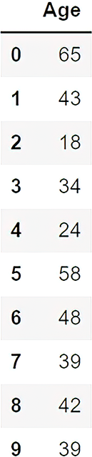
Figure 6.7 A sample set of differentially private synthetic tabular data

What are we doing in listing 6.8? We generated ten different synthetic data records using the normalized synthetic histogram that we produced in listing 6.7. That means we generated completely new synthetic data records using the properties of the normalized synthetic histogram. Now we have two different datasets: the original dataset and the synthetically produced dataset.

Now let’s compare the statistical properties of the synthetic data and the original data using histograms, as shown in listings 6.9 and 6.10.

Listing 6.9 The histogram of the synthetic data

syn_tabular_data = pd.DataFrame(syn_tabular_data_gen(len(adult_age)), 
➥ columns=['Age'])
plt.hist(syn_tabular_data['Age'], bins=age_domain)
plt.ylabel('The number of people (Frequency) - Synthetic')
plt.xlabel('Ages')

This code produces a histogram of the synthetic data as shown in figure 6.8.

Figure 6.8 A histogram produced using synthetic tabular data generation

To make a comparison, let’s generate a histogram of the original data.

Listing 6.10 The histogram of the original data

plt.bar(age_domain, age_histogram)
plt.ylabel('The number of people (Frequency) - True Value')
plt.xlabel('Ages')

The result may look like figure 6.9.

Figure 6.9 A histogram of the original data

If you compare the shapes of the histograms in figures 6.8 and 6.9, you’ll see that they are extremely similar. In other words, the synthetic data that we produced has the same statistical properties as the original data. Interesting, isn’t it?

6.3.3 DP synthetic multi-marginal data generation

The last section introduced an approach for generating privacy-preserving single- column synthetic tabular data from a synthetic histogram data representation using DP. But most real-world datasets consist of multiple-column tabular data. How can we tackle this problem?

A straightforward solution is to generate synthetic data for each column of a multiple-column tabular data using our previously described approach and then combine all the synthetic single-column tabular data together. This solution looks easy, but it does not reflect the correlations between those columns. For instance, in the US Census dataset, age and marital status are intuitively highly correlated to each other. What should we do in such cases?

We could consider multiple columns altogether. For instance, we could count how many people are 18 years old and never married, how many are 45 years old and divorced, how many are 90 years old and become widows, and so forth. Then we could calculate the probability of each case using the previous approach and sample the synthetic data from the simulated probability distribution. We’ll call this result synthetic multi-marginal data.

Let’s implement this idea on the US Census dataset containing age and marital status.

Listing 6.11 The 2-way marginal representation

two_way_marginal_rep = adult.groupby([0, 5]).size().
➥ reset_index(name = 'count')
two_way_marginal_rep

The 2-way marginal representation of the original dataset is shown in figure 6.10. Remember, column 0 is the age, and column 5 is the marital status. As you can see in the second row (index 1), 393 people are never married and age 17.

Figure 6.10 A snapshot of a 2-way marginal representation of the original dataset

We have 396 categories like this for each marital status and age combination. Once we generate a 2-way marginal dataset like this, we can use the Laplace mechanism to make it differentially private.

Listing 6.12 The differentially private 2-way marginal representation

dp_two_way_marginal_rep = laplace_mechanism(two_way_marginal_rep["count"],
➥ 1, 1)
dp_two_way_marginal_rep

The result of the 2-way marginal representation is shown in figure 6.11. As you can see, we have generated a differentially private value for all 396 categories.

Figure 6.11 A snapshot of a differentially private 2-way marginal representation

Now we can use our proposed approach to generate synthetic multi-marginal data that includes age and marital status. The following listing uses the 2-way marginal representation produced in listing 6.12 to generate a synthetic dataset.

Listing 6.13 Generating synthetic multi-marginal data

dp_two_way_marginal_rep_preprocessed = np.clip(dp_two_way_marginal_rep,
➥ 0, None)
dp_two_way_marginal_rep_normalized = dp_two_way_marginal_rep_preprocessed / 
➥ np.sum(dp_two_way_marginal_rep_preprocessed)
dp_two_way_marginal_rep_normalized
 
age_marital_pairs = [(a,b) for a,b,_ in 
➥ two_way_marginal_rep.values.tolist()]
list(zip(age_marital_pairs, dp_two_way_marginal_rep_normalized))
 
set_of_potential_samples = range(0, len(age_marital_pairs))
 
n = laplace_mechanism(len(adult), 1.0, 1.0)
 
generating_synthetic_data_samples = np.random.choice(
➥ set_of_potential_samples, int(max(n, 0)), 
➥ p=dp_two_way_marginal_rep_normalized)
synthetic_data_set = [age_marital_pairs[i] for i in 
➥ generating_synthetic_data_samples]
 
synthetic_data = pd.DataFrame(synthetic_data_set, 
➥ columns=['Age', 'Marital status'])
synthetic_data

The resulting synthetically produced 2-way marginal dataset is shown in figure 6.12.

Figure 6.12 A snapshot of a synthetically produced 2-way marginal dataset

Let’s compare the statistical properties of the synthetic data and the original data. First, let’s compare the histograms of the age data.

Listing 6.14 The histogram produced using synthetic multi-marginal data

plt.hist(synthetic_data['Age'], bins=age_domain)
plt.ylabel('The number of people (Frequency) - Synthetic')
plt.xlabel('Ages')

The histogram of the synthetic data is shown in figure 6.13.

Figure 6.13 A histogram produced using synthetically generated multi-marginal data

To compare the results, we’ll use the following code (the same as in listing 6.10) to generate a histogram of the original data.

Listing 6.15 The histogram of the original data

plt.bar(age_domain, age_histogram)
plt.ylabel('The number of people (Frequency) - True Value')
plt.xlabel('Ages')

The histogram of the original data is shown in figure 6.14. By simply looking at their shapes and how data points are distributed, we can quickly conclude that the two histograms in figures 6.13 and 6.14 are similar.

Figure 6.14 A histogram of the original data

We’ve looked at how age is distributed, but what about marital status? Let’s compare the distribution of the marital status data.

Listing 6.16 The statistics of the original data

adult_marital_status = adult[5].dropna()
adult_marital_status.value_counts().sort_index()

The results are shown in figure 6.15.

Figure 6.15 Summary of statistics of the original data

The next listing will summarize marital status data in the original dataset.

Listing 6.17 The statistics of the synthetic data

syn_adult_marital_status = synthetic_data['Marital status'].dropna()
syn_adult_marital_status.value_counts().sort_index()

Figure 6.16 shows the summary of synthetically produced data. As you can see, the marital status of the differentially private synthetic multi-marginal data looks similar to the original data (but is not the same).

Figure 6.16 Summary of statistics of the synthetically produced marital status data

Once again, we can conclude that instead of using the original data, we can use synthetically produced data to do the same tasks while preserving the privacy of the original data.

We have looked at generating synthetic histogram data representations that satisfy DP, and we have walked through using the differentially private synthetic histogram representations to generate privacy-preserving synthetic single-column tabular data and multi-marginal data. But wait! How can we deal with a large dataset with more than two or three columns and tons of records? We’ll find out the answers to that next. The next section will look at a more complex case study to demonstrate how we can apply data anonymization and DP for privacy-preserving synthetic data generation for ML.

Exercise 1: Try it yourself

In listing 6.11 we looked at a the 2-way marginal representation with age and marital status. As discussed, age and marital status are highly correlated, and we wanted to see whether the synthetically produced data also followed a similar distribution. Now try following the same steps for the education and occupation columns to see whether you have similar results.

Hint: In the original dataset, education is in column 3, and column 6 is the occupation. Start by changing the columns in listing 6.11 as follows:

adult.groupby([3, 6]).size().reset_index(name = 'count') 

Then follow all the steps.

Exercise 2: Try it yourself

Repeat the same process but for 3-way marginal representation with 3-column data. For example, you might consider age, occupation, and marital status as the 3-way representation.

6.4 Case study on private synthetic data release via feature-level micro-aggregation

Now that we have discussed different approaches to generating synthetic data, let’s walk through a case study on designing a private synthetic data-release mechanism via a feature-level micro-aggregation method. Sound too technical? Don’t worry, we’ll go through the details step by step.

First, though, recall that DP is a mechanism that provides a strong privacy guarantee to protect individual data records (as we discussed in chapter 2). In this case study, we will discuss a privacy-preserving synthetic data generation method under DP guarantee that will work with multiple ML tasks. It was developed on differentially private generative models of clustered data to generate synthetic datasets. In the latter part of this section, we will show you how effective this method is compared to some existing approaches, and how it improved the utility compared to other methods.

Before we look at the details of the case study, let’s first recap some of the basics. Usually, designing a powerful privacy-preserving synthetic data generation method for ML comes with many challenges. First, a privacy-preserving method usually introduces perturbation to data samples that hurts the utility of the data. Mitigating the perturbation so that you reach a certain level of utility is not an easy task. Second, ML can be represented in many different tasks, like classification, regression, and clustering. An effective synthetic data generation method should be applicable to all these various tasks. Third, some data can come in the form of very complex distributions. In that case, it is hard to form an accurate generator based on the whole data distribution.

In the past, people have proposed several private synthetic data-release algorithms [4], [5]. One of the common approaches is to utilize noisy histograms to release synthetic data, but most of them are designed to work with categorical feature variables. On the other hand, some algorithms are designed to generate synthetic data under a statistical model with some preprocessing on the original dataset. However, they usually only generate synthetic data based on the whole data distribution.

In this study, we will focus on how we can generate synthetic data while maintaining statistical characteristics similar to the original dataset while ensuring data owners have no privacy concerns.

Now that you have a basic understanding of what we’re going to do, let’s dig into the details.

6.4.1 Using hierarchical clustering and micro-aggregation

An essential part of our methodology that we’ll build on is hierarchical clustering. In essence, hierarchical clustering is an algorithm that clusters input samples into different clusters based on the proximity matrix of samples. This proximity matrix represents the distance between each cluster. In this case, we’ll use agglomerative hierarchical clustering [6], a bottom-up approach, which starts by assigning each data sample to its own group and merging the pairs of clusters that have the smallest distance, until there is only a single cluster left.

As discussed in section 6.2, k-anonymity can be used to anonymize data. Here, we will use a data anonymization algorithm called micro-aggregation that can achieve k-anonymity. The micro-aggregation approach we are referring to here is a simple heuristic method called maximum distance to average record (MDAV) proposed by Domingo-Ferrer et al. [7]. The idea is to separate samples into clusters, and each cluster contains exactly k records except the last one. Records in the same cluster are supposed to be as similar as possible in terms of distance. In addition, each record in the cluster will be replaced by a representative record for the cluster to complete the data anonymization.

6.4.2 Generating synthetic data

In this synthetic data generation mechanism, four main components operate collectively to generate synthetic data that satisfies DP:

• Data preprocessing—Combines independent feature sets and feature-level micro-aggregation to produce data clusters that describe the data more generally.

• Statistic extraction—Extracts the representative statistical information of each data cluster.

• DP sanitizer—Adds differential private noise on extracted statistical information.

• Data generator—Generates synthetic data sample by sample from the perturbed generative model.

These four components are shown in figure 6.17.

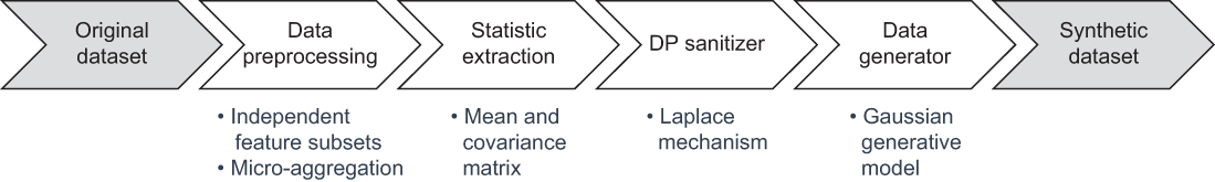
Figure 6.17 Different components of the synthetic data generation algorithm

How data preprocessing works

In data preprocessing, we use micro-aggregation as the clustering method for samples in full feature dimension (samples that cover all the features we are interested in). Instead of replacing records with a representative record, we will use a differentially private generative model to model each cluster. However, there are a few challenges here.

When modeling the output clusters from MDAV, some clusters may carry correlations that may not exist in the actual data distribution. This false feature correlation may apply unnecessary constraints when modeling the data clusters, and this may lead the synthetic data into a different shape. On the other hand, we know that a noise variance is usually introduced by DP. Intuitively, the less the noise introduced by DP, the higher the utility. Hence, reducing the DP mechanism’s noise also helps us improve the data’s utility. To address these adverse effects, we can sample data not only at the sample level but also at the feature level.

Here is how feature-level and sample-level clustering work:

• Feature-level clustering—Whenever we have a numerical dataset D⁽n^×d⁾, we can divide these d data features into m independent feature sets using agglomerative hierarchical clustering. Here, a distance function that converts Pearson correlation to distance can be used to form the proximity matrix in hierarchical clustering. Features with higher correlation should have lower distance, and lower correlation corresponds to a higher distance. This approach will help us to ensure the features in the same set are more correlated to each other and less correlated to features in the other feature sets.

• Sample-level clustering—Once we have the output of feature-level clustering, we split data on the feature level and then apply micro-aggregation to each data segment. The idea is to assign the homogeneous samples to the same cluster, which will help us preserve more information from the original data. The sensitivity of each sample cluster can also be potentially reduced compared to the global sensitivity. This reduction will involve less noise in the DP mechanism. In other words, it enhances the data’s utility under the same level of privacy guarantee.

The concepts behind generating synthetic data

The micro-aggregation process outputs several clusters having at least k records each. Assuming each cluster forms a multivariate Gaussian distribution, the mean (μ) and covariance matrix (Σ) are computed for each cluster c. Then the privacy sanitizer adds the noise on μ and Σ to ensure that the model is satisfied with DP. Finally, the generative model is built. The complete process of generating synthetic data is illustrated in figure 6.18.

Figure 6.18 How the synthetic data generator works. Here μ represents the mean and Σ is the covariance matrix computed for each cluster.

In figure 6.18, the original multivariate Gaussian model is parameterized by the mean (μ) and covariance matrix (Σ). It is noteworthy that the privacy sanitizer outputs two parameters, μ_DP and Σ_DP, that are protected by DP. Hence, the multivariate Gaussian model that is parameterized by μ_DP and Σ_DP is also protected by DP. In addition, depending on the postprocessing invariance of DP, all the synthetic data derived from DP multivariate Gaussian models is also protected by DP.

6.4.3 Evaluating the performance of the generated synthetic data

To evaluate the performance of the proposed method, we have implemented it in Java. Yes, this time it’s Java. The complete source code, dataset, and evaluation tasks are available in the book’s GitHub repository: https://github.com/nogrady/PPML/blob/main/Ch6/PrivSyn_Demo.zip.

We generated different synthetic datasets and performed experiments under different cluster sizes (k) and privacy budgets (ε). The setting of ε varies from 0.1 to 1 and cluster size varies: k = 25, 50, 75, 100. For each synthetic dataset, we looked at the performance on three general ML tasks: classification, regression, and clustering. To accomplish these tasks, we have two different experiment scenarios using different synthetic and original data combinations.

• Experiment scenario 1—Original data is used for training, and synthetic data is used for testing.

  The ML model trains on the original datasets and tests the generated synthetic datasets. For each experimental dataset, 30% of the samples are used as the seed dataset to generate the synthetic dataset, and 70% is used as original data to train the model. Generated synthetic data is used for testing.

• Experiment scenario 2—Synthetic data is used for training, and original data is used for testing.

  The ML model trains on the synthetic datasets and tests on the original datasets. For each experimental dataset, 80% of the samples are used as a seed dataset to generate the synthetic dataset, and 20% is used as original data to test the model.

Datasets used for the experiments

For this performance evaluation, we used three datasets from the UCI Machine Learning Repository [8] and LIBSVM data repository to examine the performance of the different algorithms. All the features in the dataset were scaled to [-1,1]:

• Diabetes dataset—This dataset contains diagnostic measurements of patient records with 768 samples and 9 features, including patient information such as blood pressure, BMI, insulin level, and age. The objective is to identify whether a patient has diabetes.

• Breast cancer dataset—This dataset was collected from clinical cases for breast cancer diagnosis. It has 699 samples and 10 features. All the samples are labeled as benign or malignant.

• Australian dataset—This is the Australian credit approval dataset from the StatLog project. Each sample is a credit card application, and the dataset contains 690 samples and 14 features. The samples are labeled by whether the application is approved or not.

Performance evaluation and the results

As discussed, we are interested in three main ML tasks for the evaluation of synthetic data: classification, regression, and clustering.

A support vector machine (SVM) was used for the classification task. In each training phase, we used grid search and cross-validation to choose the best parameter combination for the SVM model. In terms of selecting the best performing SVM model, the F1 score was utilized. The model with the highest F1 score was used to test classification accuracy.

For the regression task, linear regression was used as the regressor. The evaluation metric of regression is mean squared error (MSE).

Finally, k-means clustering was used as the clustering task. As you learned in the previous chapters, clustering is an unsupervised ML task that groups similar data. Unlike the preceding classification and regression tasks, all data in the original dataset is considered the seed for synthetic data in clustering. The k-means algorithm is applied on both the original and synthetic datasets, and both result in two clusters that present the binary class in experimental datasets. In each experiment, k-means runs 50 times with different centroid seeds, and it outputs the best case of 50 consecutive runs.

The results of the three ML tasks are shown in figures 6.19, 6.20, and 6.21. You can see that when ε ranges from 0.1 to 0.4, the performance of each k increases rapidly, but the peak performance is not always coming from a fixed k value. For example figure 6.19 (e) has a local optimal point when k = 50, and figures 6.21 (a) and figure 6.21 (c) have a local optimal point when k = 75.

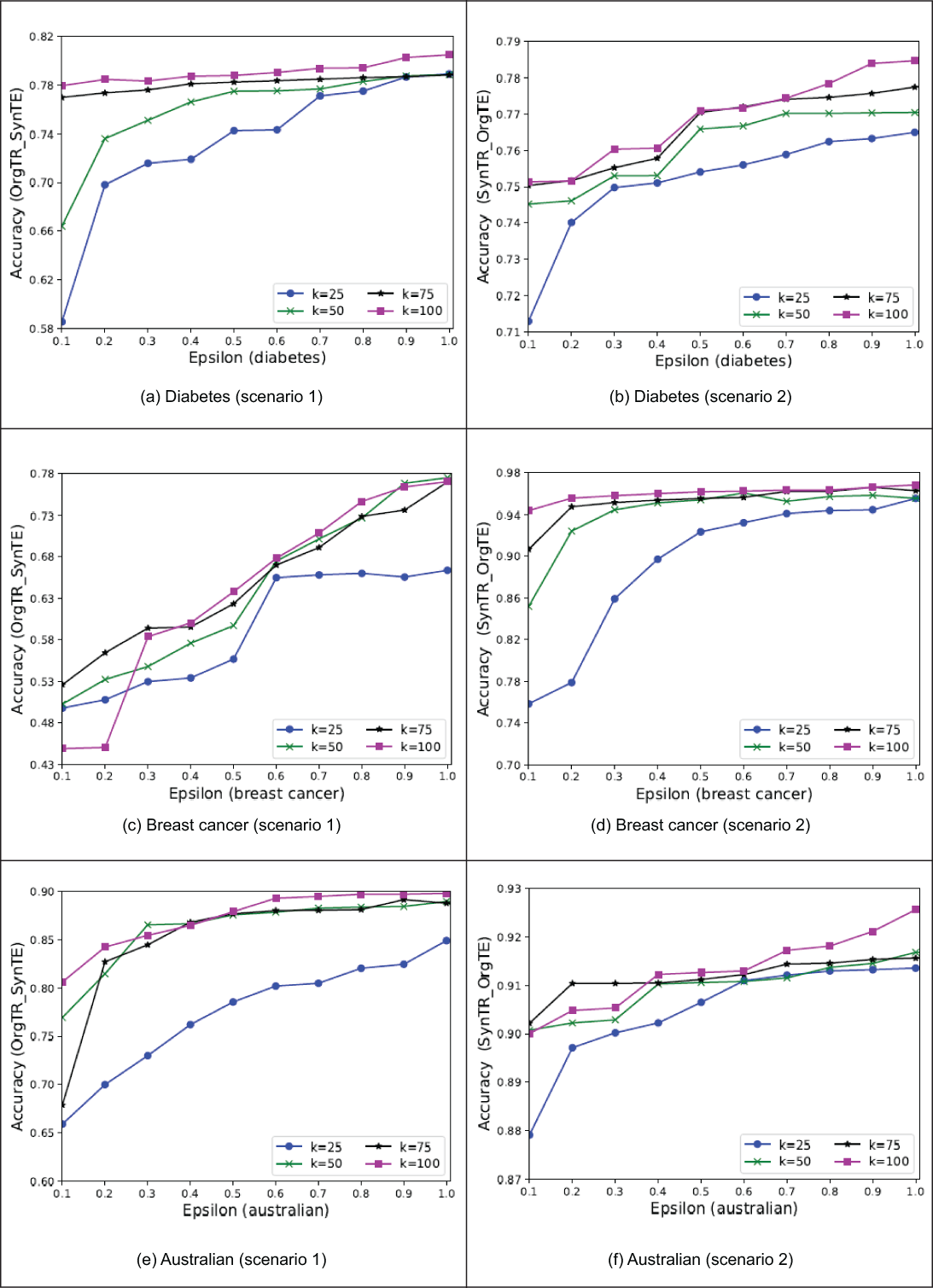
Figure 6.19 Experimental results of task 1 (SVM) with the two different experiment scenarios

Figure 6.20 Experimental results of task 2 (linear regression) with the two different experiment scenarios

Figure 6.21 Experimental results of task 3 (k-means clustering)

Theoretically speaking, a small ε value usually introduces more noise to the synthetic data than a greater ε value, which brings more randomness. Comparing the two scenarios in the case of regression (figure 6.20), the randomness reflected in scenario 2 has much less MSE than in scenario 1, when the privacy budget was small. This is due to the testing data in scenario 1 having differentially private noise, and the testing data in scenario 2 not having the noise in it. Whenever ε > 0.4, the performance increase is somewhat steady, and when k = 100, the clustering method always outperforms the other k values under the same privacy budget. It is also noteworthy that when k = 25, the overall performance is much lower than for the other k values. That’s because when we form a multivariate Gaussian generative model on a cluster that only contains a few data samples, the calculated mean and the covariance matrix can be biased. The cluster cannot reflect the data distribution very well. Thus, k should be a moderate value to form the multivariate Gaussian generative model. A greater k value can also make the model converge faster than a smaller k, as in figures 6.19 (a), 6.19 (d), 6.20 (a), and 6.21 (a).

Summary

• Synthetic data is artificial data that is generated from the original data and that keeps the original data’s statistical properties and protects the original data’s private information.

• The synthetic data generation process involves various steps, including outlier detection, a normalization function, and building the model.

• A privacy test is used to ensure that the generated synthetic data satisfies certain predefined privacy guarantees.

• K-anonymity is a good approach for generating anonymized synthetic data to mitigate re-identification attacks.

• While k-anonymity makes it harder to re-identify individuals, it also has some drawbacks, which leads to other anonymization mechanisms such as l-diversity.

• A synthetic representation of a dataset can capture statistical properties of the original dataset, but most of the time it will not have the same shape as the original dataset.

• We can use a synthetic histogram to generate synthetic tabular data.

• A synthetic representation can be used to generate a synthetic dataset with the same statistical properties and shape as the original dataset.

• We can generate differentially private synthetic data by applying the Laplace mechanism to the synthetic representation generator and then use the differentially private synthetic representation generator.

• We can generate differentially private synthetic data that satisfies k-anonymity by applying micro-aggregation techniques to synthetic data generation.