9 Compressive privacy for machine learning

This chapter covers

• Understanding compressive privacy
• Introducing compressive privacy for machine learning applications
• Implementing compressive privacy from theory to practice
• A compressive privacy solution for privacy-preserving machine learning

In previous chapters we’ve looked into differential privacy, local differential privacy, privacy-preserving synthetic data generation, privacy-preserving data mining, and their application when designing privacy-preserving machine learning solutions. As you’ll recall, in differential privacy a trusted data curator collects data from individuals and produces differentially private results by adding precisely computed noise to the aggregation of individuals’ data. In local differential privacy, individuals privatize their own data by perturbation before sending it to the data aggregator, which eliminates the need to have a trusted data curator collect the data from individuals. In data mining, we looked into various privacy-preserving techniques and operations that can be used when collecting information and publishing the data. We also discussed strategies for regulating data mining output. Privacy- preserving synthetic data generation provides a promising solution for private data sharing, where synthetic yet representative data can be generated and then shared among multiple parties safely and securely.

As you can see, most of the techniques we have discussed are based on the definition of differential privacy (DP), which does not make any assumptions about the abilities of the adversaries, thus providing an extremely strong privacy guarantee. However, to enable this strong privacy guarantee, DP-based mechanisms usually add excessive noise to the private data, causing a somewhat inevitable utility drop. This prevents DP approaches from being applied for many real-world applications, and especially for practical applications using machine learning (ML) or deep learning. This prompts us to explore other perturbation-based approaches to privacy preservation. Compressive privacy (CP) is one alternative approach we can look into. In this chapter we will explore the concept, mechanisms, and applications of compressive privacy.

9.1 Introducing compressive privacy

Compressive privacy (CP) is an approach that perturbs the data by projecting it to a lower-dimensional hyperplane via compression and dimensionality-reduction (DR) techniques. To better understand the concept and benefits of CP, let’s compare it with the idea of differential privacy (DP), which we discussed in chapter 2.

According to the definition of DP, a randomized algorithm M is said to be ε-DP of the input data if it satisfies Pr[M(D) ∈ S] ≤ e^ε ∙ Pr[M(D') ∈ S] for all S ∈ Range(M) and all datasets D and D' differing by one item, where Range(M) is the output set of M. In other words, the idea behind DP is that if the effect of making an arbitrary single change or substitution in a database is small enough, the query result cannot be used to infer much about any single individual, and it therefore provides privacy. As you can see, DP guarantees that the distribution of the query result from a dataset should be indistinguishable (modulo by a factor of e ^ε) whether or not any single item in that dataset is changed. The DP definition does not make any assumptions about adversaries in advance. For instance, adversaries could have unbounded auxiliary information and unlimited computing resources, and DP mechanisms can still provide privacy guarantees under this definition of DP.

This shows the bright side of DP—it provides strong privacy guarantees via rigorous theoretical analysis. However, the DP definition and mechanisms do not make any assumptions about utility. As such, DP mechanisms usually cannot promise good performance in terms of utility. This is particularly true when applying DP approaches to real-world applications that require complex calculations, such as data mining and machine learning. That’s why we also need to explore other privacy-enhancing techniques that consider utility while relaxing the theoretical privacy guarantees somewhat. CP is one such alternative that can be used with practical applications.

Unlike DP, the CP approach allows the query to be tailored to the known utility and privacy tasks. Specifically, for datasets that have samples with two labels, a utility label and a privacy label, CP allows the data owner to project their data to a lower dimension in a way that maximizes the accuracy of learning for the utility labels while decreasing the accuracy of learning for the privacy labels. We will discuss these labels when we get into the details. It is also noteworthy that, although CP does not eliminate all data privacy risks, it offers some control over the misuse of data when the privacy task is known. In addition, CP guarantees that the original data can never be fully recovered, mainly due to the dimensionality reduction.

Now let’s dig into how CP works. Figure 9.1 illustrates the threat model of CP. The adversaries are all the data users with full access to the public datasets (e.g., background and auxiliary information).

Figure 9.1 The threat model of compressive privacy. The real challenge is balancing the utility and privacy tradeoff.

In this scenario, let’s assume that the privacy task is a two-class {+,-} classification problem (utility tasks are independent of the privacy task), and X₊, X_- are two public datasets. Suppose X_S is the private data of the data owner, where s ∈{+,-} is its original class (privacy task) and t ∈ {+,-} is its expected class (privacy task) after applying the CP perturbation. The data owner could publish z (the perturbed version of X_S) using the CP mechanisms. However, there could also be an adversary out there, using their approach z' = A(z, X₊, X_-) to inference the original (privacy task) class s. Thus, what we want to achieve here is to minimize the probability difference, |Pr (z' = +|z) - P r (z' = -|z)|, so that the adversary cannot learn any valuable information.

In figure 9.1 Alice (the data owner) has some private data, and she wants to publish it for a utility task. Let’s say the utility task is to allow a data user to perform an ML classification with the data. Since it contains personal information, Alice can perturb the data using CP. Whenever Bob (the data user) wants to use this compressed data, he needs to recover the information, which he can do using the statistical properties of a publicly available dataset in a similar domain (which we call the utility task feature space). The problem is that someone else, Eve (an adversary), might also use the compressed data and try to recover it using another publicly available dataset, which might lead to a privacy breach. Thus, the real challenge with CP is balancing this utility/privacy tradeoff. We can compress data to perform the utility task, but it still needs to be challenging for someone to recover the data to identify personal information.

The following section will walk you through several useful components that enable CP for privacy-preserving data sharing or ML applications.

9.2 The mechanisms of compressive privacy

An important building block of CP is the supervised dimensionality reduction technique, which relies on data labels. Principal component analysis (PCA) is a widely used method that aims to project the data on the principal components with the highest variance, thus preserving most of the information in the data while reducing the data dimensions. We briefly discussed this in section 3.4.1, but let’s recap it quickly.

9.2.1 Principal component analysis (PCA)

Let’s first understand what principal components are. Principal components are new variables constructed as linear combinations of the initial variables in a dataset. These combinations are created in such a way that the new variables are uncorrelated, and most of the information within the initial variables is compressed into the first components (which is why we call it compressive). So, for instance, when 10-dimensional data gives you 10 principal components, PCA tries to put the maximum possible information in the first component, the maximum remaining information in the second component, and so on. When you organize information in principal components like this, you reduce dimensionality without losing much of the critical information.

Let’s consider a dataset with N training samples {x₁, x₂, ..., x_N}, where each sample has M features (x_i ∈ ℝ^M). PCA performs something called spectral decomposition of the center-adjusted scatter matrix such that

where μ is the mean vector, and Λ = diag(λ₁, λ₂, ..., λ_M) is a diagonal matrix of eigenvalues with eigenvalues arranged in a monotonically decreasing order (i.e., λ₁ ≥ λ₂ ≥ ⋯ ≥ λ_M).

Here, the matrix U = [u₁,u₂, ..., u_M] is an M × M unitary matrix where u_j denotes the jth eigenvector of the scatter matrix mentioned previously. For PCA, we retain the m principal components corresponding to the m highest eigenvalues to obtain the projection matrix U_m. Once the projection matrix is found, you can find the reduced dimension feature vector as follows:

As you can see, the parameter m determines to what extent the signal power is retained after dimensionality reduction.

9.2.2 Other dimensionality reduction methods

Now that you know how PCA works, by projecting the data on principal components, let’s look at a few other approaches that can be used for different ML classification tasks. Because the same dataset could be utilized in different classification problems, let’s define a classification problem as c which has a unique set of labels associated with the corresponding training samples x_i. Without loss of generality, the dataset could be utilized for a single utility target U and a single privacy target P.

For example, suppose an ML algorithm is trained with a dataset of face images. The utility target is to identify the faces, whereas the privacy target is to identify the person. In this case, each training sample x_i has two labels ∈ {1, 2, ..., L^u} and ∈ {1, 2, ..., L^p}. L^u and L^p are the numbers of classes of the utility target and the privacy target, respectively.

Based on Fisher’s linear discriminant analysis [1], [2], given a classification problem, the within-class scatter matrix of its training samples contains most of the noise information, while the between-class scatter matrix of its training samples contains most of the signal information. We can define the within-class scatter matrix and the between-class scatter matrix for the utility target as follows,

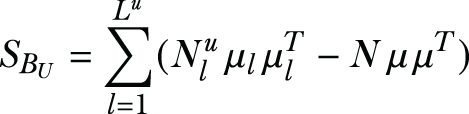
where is the mean vector of all training samples belonging to class l, and N^u_l is the number of training samples belonging to class l of the utility target.

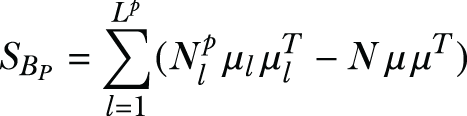
Similarly, for the privacy target, the within-class scatter matrix and the between-class scatter matrix are defined as

Suppose we let W be a K × M projection matrix, in which K < M. Given a testing sample x, ∙ W is its subspace projection. The framework that we are going to explore here combines the advantages of two eigenvalue decomposition-based dimensionality reduction (DR) techniques: DCA (utility-driven projection) [3] and MDR (privacy emphasized projection) [4]. Let’s quickly look into those:

• Discriminant component analysis (DCA)—DCA involves searching for the projection matrix W ∈ R^M×K,

  

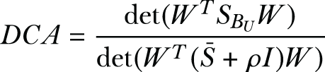
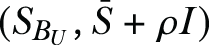
  where det(.) is the determinant operator, ρI is a small regularization term added for numerical stability, and .

  The optimal solution to this problem can be derived from the first K principal generalized eigenvectors of the matrix pencil .

• Multiclass discriminant ratio (MDR)—MDR considers both the utility target and the privacy target, which is defined as

  

  where ρI is a small regularization term added for numerical stability. The optimal solution to MDR can be derived from the first K principal generalized eigenvectors of the matrix pencil .

With those basics and mathematical formulations, let’s look at how we can implement CP techniques in Python.

9.3 Using compressive privacy for ML applications

So far we’ve discussed the theoretical background of different CP mechanisms. Let’s implement these techniques in a real-world face-recognition application. Face recognition has been a problem of interest in machine learning (ML) and signal processing for over a decade due to its various use cases ranging from simple online image searches to surveillance.

With the current privacy requirements, a real-world face-recognition application has to ensure that there won’t be any privacy leaks from the data itself. Let’s investigate a couple of different CP methods to see how we can ensure both the utility of the face recognition application and the privacy of the reconstructed image. We’ll need to compress the face image before submitting it to the facial-recognition application such that the application can still identify the face. However, someone else should not be able to distinguish the image simply by looking at it or be able to reconstruct the original image. For our experiments, we will employ three different face datasets. The source code for these hands-on experiments is available for download at the book’s GitHub repository: https://github.com/nogrady/PPML/tree/main/Ch9.

• Yale Face Database—The Yale Face Database contains 165 grayscale images of 15 individuals and is publicly available from http://cvc.cs.yale.edu/cvc/projects/yalefaces/yalefaces.html.

• Olivetti faces dataset—This dataset contains 400 grayscale face images of 40 different people taken between April 1992 and April 1994 at AT&T Laboratories Cambridge. The dataset can be downloaded from https://scikit-learn.org/0.19/datasets/olivetti_faces.html.

• Glasses dataset—We derived this dataset from a combination of the Yale and Olivetti datasets by selectively choosing the subjects who are wearing glasses. In this case, the dataset contains 300 images. Half of the images are of people with glasses, and the other half are people without glasses.

For the Yale and Olivetti datasets, the task of recognizing individuals from the face images will be our utility (our target application), whereas reconstructing the image will be our privacy target. One use case scenario would be an “entity” that wants to build a face recognition algorithm using sensitive face images provided by users for training. But in this scenario, people are usually hesitant to share their face images unless they are changed so that no one can recognize the person in the image.

For simplicity, we can assume that the entity wishing to build the face recognition classifier is a service operator, but this operator could be malicious and could be trying to reconstruct the original images from the training data received from users.

For the glasses dataset, we have two different classes (with and without glasses). The utility of our application will be to identify whether the person is wearing a pair of glasses or not; the privacy target will again be the reconstruction of the image.

9.3.1 Implementing compressive privacy

Now let’s get to work! We’ll use the Yale dataset and see how we can use CP techniques in our facial recognition application. First, you’ll need to load some modules and the dataset. Note that discriminant_analysis.py is a module that we developed for PCA and DCA methods. Refer to the source code for more information.

Note You can just use the cleaned version of the Yale dataset, which is available in the code repository: https://github.com/nogrady/PPML/tree/main/Ch9.

Listing 9.1 Loading modules and the dataset

import sys
sys.path.append('..');
import numpy as np
from discriminant_analysis import DCA, PCA
from sklearn.svm import SVC
from sklearn.model_selection import GridSearchCV
from sklearn.model_selection import train_test_split
from matplotlib.pyplot import *
 
data_dir = './CompPrivacy/DataSet/Yale_Faces/';    ❶
X = np.loadtxt(data_dir+'Xyale.txt');
y = np.loadtxt(data_dir+'Yyale.txt');

❶ Load the dataset.

You can run the following command to see what the dataset looks like:

print('Shape of the dataset: %s' %(X.shape,))

As you can see from the output, the dataset contains 165 images, where each image is 64 x 64 (which is why we get 4,096).

Shape of the dataset: (165, 4096)

Now let’s review a couple of images in the dataset. Because the dataset contains 165 different images, you can run the code in the following listing to pick four different images randomly. We are using the randrange function to randomly choose images. To show the images in the output, we are using the displayImage routine and subplot with four columns.

Listing 9.2 Loading a few images from the dataset

def displayImage(vImage,height,width):             ❶
    mImage = np.reshape(vImage, (height,width)).T
    imshow(mImage, cmap='gray')
    axis('off')
 
for i in range(4):                                 ❷
    subplot(1,4,i+1)
    displayImage(X[randrange(165)], height, width)
 
show()

❶ Define a function to show the images.

❷ Randomly select four different images from the dataset.

The output will look something like figure 9.2, though you will get different random face images.

Figure 9.2 A set of sample images from Yale dataset

Now that you know what kind of data we are dealing with, let’s implement different CP technologies with this dataset. We are particularly looking at implementing principal component analysis (PCA) and discriminant component analysis (DCA) with this dataset. We have developed and wrapped the core functionality of PCA and DCA into the discriminant_analysis.py class, so you can simply call it and initialize the methods.

Note Discriminant_analysis.py is a class file that we developed to cover the PCA and DCA methods. You can refer to the source code of the file for more information: https://github.com/nogrady/PPML/blob/main/Ch9/discriminant_analysis.py.

The DCA object is initialized with two parameters: rho and rho_p. You’ll recall that we discussed these parameters (ρ and updated ρ) in section 9.2.2. The code we use will first define and initialize these values along with a set of dimensions that we’ll need to project the image data in order to see the results.

We’ll start by setting rho = 10 and rho_p = -0.05, but later in this chapter you’ll learn about the important properties of these parameters and how different values will affect privacy. For now we’ll just focus on the training and testing part of the algorithm.

Setting ntests = 10 means that we will do the same experiment 10 times to average the final result. You can set this value to any number, but the higher, the better. The dims array defines the number of dimensions that we will use. As you can see, we will be starting with few dimensions, such as 2, and then move to more dimensions, such as 4,096. Again, you can try setting your own values for this.

rho = 10; 
rho_p = -0.05;
ntests = 10;
dims = [2,5,8,10,14,39,1000,2000,3000,4096];
 
mydca = DCA(rho,rho_p);
mypca = PCA();

Once these values are defined, the mypca and mydca objects are trained with the following code, after the dataset is split into train and test sets. Xtr is the training data matrix (training set), while ytr is the training label vector. The fit command learns some quantities from the data, particularly the principal components and the explained variance.

Xtr, Xte, ytr, yte = train_test_split(X,y,test_size=0.1,stratify=y);
mypca.fit(Xtr);
mydca.fit(Xtr,ytr);

Thereafter, the projections of the data can be obtained as follows:

Dtr_pca = mypca.transform(Xtr);
Dte_pca = mypca.transform(Xte);
Dtr_dca = mydca.transform(Xtr);
Dte_dca = mydca.transform(Xte);   
print('Principal and discriminant components were extracted.')

For each dimension that we are interested in (2, 5, 8, 10, 14, 39, 1000, etc.), the projection matrix D can be found, and then the image data can be reconstructed as Xrec:

D = np.r_[Dtr_pca[:,:dims[j]],Dte_pca[:,:dims[j]]];   ❶
Xrec = np.dot(D,mypca.components[:dims[j],:]);
 
D = np.r_[Dtr_dca[:,:dims[j]],Dte_dca[:,:dims[j]]];   ❷
Xrec = mydca.inverse_transform(D,dim=dims[j]);

❶ Reconstruct the data using PCA technique.

❷ Reconstruct the data using DCA technique.

When we put all this together, the complete code looks like the following listing.

Listing 9.3 The complete code to reconstruct an image and calculate the accuracy

import sys
sys.path.append('..');
import numpy as np
from random import randrange
from discriminant_analysis import DCA, PCA
from sklearn.svm import SVC
from sklearn.model_selection import GridSearchCV
from sklearn.model_selection import train_test_split
from matplotlib.pyplot import *
 
def displayImage(vImage,height,width):
    mImage = np.reshape(vImage, (height,width)).T
    imshow(mImage, cmap='gray')
    axis('off')
 
height = 64
width = 64
 
data_dir = './CompPrivacy/DataSet/Yale_Faces/';
X = np.loadtxt(data_dir+'Xyale.txt');
y = np.loadtxt(data_dir+'Yyale.txt');
 
print('Shape of the dataset: %s' %(X.shape,))
 
for i in range(4):    
    subplot(1,4,i+1)
    displayImage(X[randrange(165)], height, width)
show()
 
 
rho = 10; 
rho_p = -0.05;
ntests = 10;
dims = [2,5,8,10,14,39,1000,2000,3000,4096];
 
mydca = DCA(rho,rho_p);
mypca = PCA();
       
svm_tuned_params = [{'kernel': ['linear'], 'C': 
➥ [0.1,1,10,100,1000]},{'kernel':
    ['rbf'], 'gamma': [0.00001, 0.0001, 0.001, 0.01], 'C': 
    ➥ [0.1,1,10,100,1000]}];
           
utilAcc_pca = np.zeros((ntests,len(dims)));
utilAcc_dca = np.zeros((ntests,len(dims)));
reconErr_pca = np.zeros((ntests,len(dims)));
reconErr_dca = np.zeros((ntests,len(dims)));
 
clf = GridSearchCV(SVC(max_iter=1e5),svm_tuned_params,cv=3);
 
for i in range(ntests):
    print('Experiment %d:' %(i+1));
    Xtr, Xte, ytr, yte = train_test_split(X,y,test_size=0.1,stratify=y);
    mypca.fit(Xtr);
    mydca.fit(Xtr,ytr);
 
    Dtr_pca = mypca.transform(Xtr);                                     ❶
    Dte_pca = mypca.transform(Xte);
    Dtr_dca = mydca.transform(Xtr);
    Dte_dca = mydca.transform(Xte);   
    print('Principal and discriminant components were extracted.')
    
    subplot(2,5,1)
    title('Original',{'fontsize':8})
    displayImage(Xtr[i],height,width)
    
    subplot(2,5,6)
    title('Original',{'fontsize':8})
    displayImage(Xtr[i],height,width)    
    
    for j in range(len(dims)):
        clf.fit(Dtr_pca[:,:dims[j]],ytr);                               ❷
        utilAcc_pca[i,j] = clf.score(Dte_pca[:,:dims[j]],yte);
        print('Utility accuracy of %d-dimensional PCA: %f' 
              %(dims[j],utilAcc_pca[i,j]));
        
        D = np.r_[Dtr_pca[:,:dims[j]],Dte_pca[:,:dims[j]]];             ❸
        Xrec = np.dot(D,mypca.components[:dims[j],:]);
        reconErr_pca[i,j] = sum(np.linalg.norm(X-Xrec,2,axis=1))/len(X);
        eigV_pca = np.reshape(Xrec,(len(X),64,64))
        print('Average reconstruction error of %d-dimensional PCA: %f' 
              %(dims[j],reconErr_pca[i,j]));
             
        clf.fit(Dtr_dca[:,:dims[j]],ytr);                               ❹
        utilAcc_dca[i,j] = clf.score(Dte_dca[:,:dims[j]],yte);
        print('Utility accuracy of %d-dimensional DCA: %f' 
              %(dims[j],utilAcc_dca[i,j]));
        
        D = np.r_[Dtr_dca[:,:dims[j]],Dte_dca[:,:dims[j]]];             ❺
        Xrec = mydca.inverse_transform(D,dim=dims[j]);
        reconErr_dca[i,j] = sum(np.linalg.norm(X-Xrec,2,axis=1))/len(X);
        eigV_dca = np.reshape(Xrec,(len(X),64,64))
        print('Average reconstruction error of %d-dimensional DCA: %f' 
              %(dims[j],reconErr_dca[i,j]));    
        
        subplot(2,5,j+2)                                                ❻
        title('DCA dim: ' + str(dims[j]),{'fontsize':8})
        displayImage(eigV_dca[i],height,width) 
        
        subplot(2,5,j+7)
        title('PCA dim: ' + str(dims[j]),{'fontsize':8})
        displayImage(eigV_pca[i],height,width)        
        
    show()
 
np.savetxt('utilAcc_pca.out', utilAcc_pca, delimiter=',')               ❼
np.savetxt('utilAcc_dca.out', utilAcc_dca, delimiter=',')
np.savetxt('reconErr_pca.out', reconErr_pca, delimiter=',')
np.savetxt('reconErr_dca.out', reconErr_dca, delimiter=',')

❶ Precompute all the components.

❷ Test the accuracy of PCA.

❸ Test the reconstruction error of PCA.

❹ Test the accuracy of DCA.

❺ Test the reconstruction error of DCA.

❻ Show the reconstructed image.

❼ Save the accuracy and reconstruction error of each cycle as a text file.

As you can see in listing 9.3, we are running the PCA and DCA reconstructions 10 times (remember we set ntests = 10), and for each case it randomly splits the dataset for training and testing. In the end, we are calculating the accuracy and reconstruction error for each dimension for both PCA and DCA. That will let us evaluate how accurately the compressed image can be reconstructed.

When you run the code, the results may look like the following. The complete output is too long to include here—we’ve just included the first few lines of the output and the reconstructed images of the first two runs in the loop.

Experiment 1:
Principal and discriminant components were extracted.
Utility accuracy of 5-dimensional PCA: 0.588235
Average reconstruction error of 5-dimensional PCA: 3987.932630
Utility accuracy of 5-dimensional DCA: 0.882353
Average reconstruction error of 5-dimensional DCA: 7157.040696
Utility accuracy of 14-dimensional PCA: 0.823529
Average reconstruction error of 14-dimensional PCA: 4048.247986
Utility accuracy of 14-dimensional DCA: 0.941176
Average reconstruction error of 14-dimensional DCA: 7164.268844
Utility accuracy of 50-dimensional PCA: 0.941176
Average reconstruction error of 50-dimensional PCA: 4142.000701
Utility accuracy of 50-dimensional DCA: 0.941176
Average reconstruction error of 50-dimensional DCA: 6710.181110
Utility accuracy of 160-dimensional PCA: 0.941176
Average reconstruction error of 160-dimensional PCA: 4190.105696
Utility accuracy of 160-dimensional DCA: 0.941176
Average reconstruction error of 160-dimensional DCA: 4189.337999
...
...

Experiment 2:
Principal and discriminant components were extracted.
...
...

If you look closely at the reproduced images in the output, compared with the originals, you’ll see that when the reduced dimensions are low, it is difficult to identify the person. For instance, if you compare the original image and the version with 5 (either PCA or DCA), it is pretty hard to identify the person from the compressed image. On the other hand, when dims = 160, you can see that the reconstructed image is getting better. That means we are preserving the privacy of sensitive data by reducing the dimensions. As you can see, in this case, DCA works much better than PCA for the dimensions 5 to 50, making it close to the original but still hard to recognize.

9.3.2 The accuracy of the utility task

You now know that when the dimensions are reduced, privacy is improved. But what about the accuracy of the utility task? If we cannot get considerable accuracy for the utility task, there is no point in using CP techniques in this scenario.

To examine how the accuracy of the utility task changes along with the reduced dimensions, we can simply increase the value of the ntests variable to the maximum value (which is 165 because we have 165 records in the dataset) and average the utility accuracy results for each dimension.

Figure 9.3 summarizes the accuracy results. If you look carefully at the DCA results, you will notice that after the dimension becomes 14, its accuracy saturates somewhere around 91%. Now look at the face image where the dimension is 14 for DCA. You will notice that it is hard to identify the person but the graph shows that the accuracy of the utility task (the facial recognition application in this case) is still high. That is how CP works, ensuring the balance between privacy and utility.

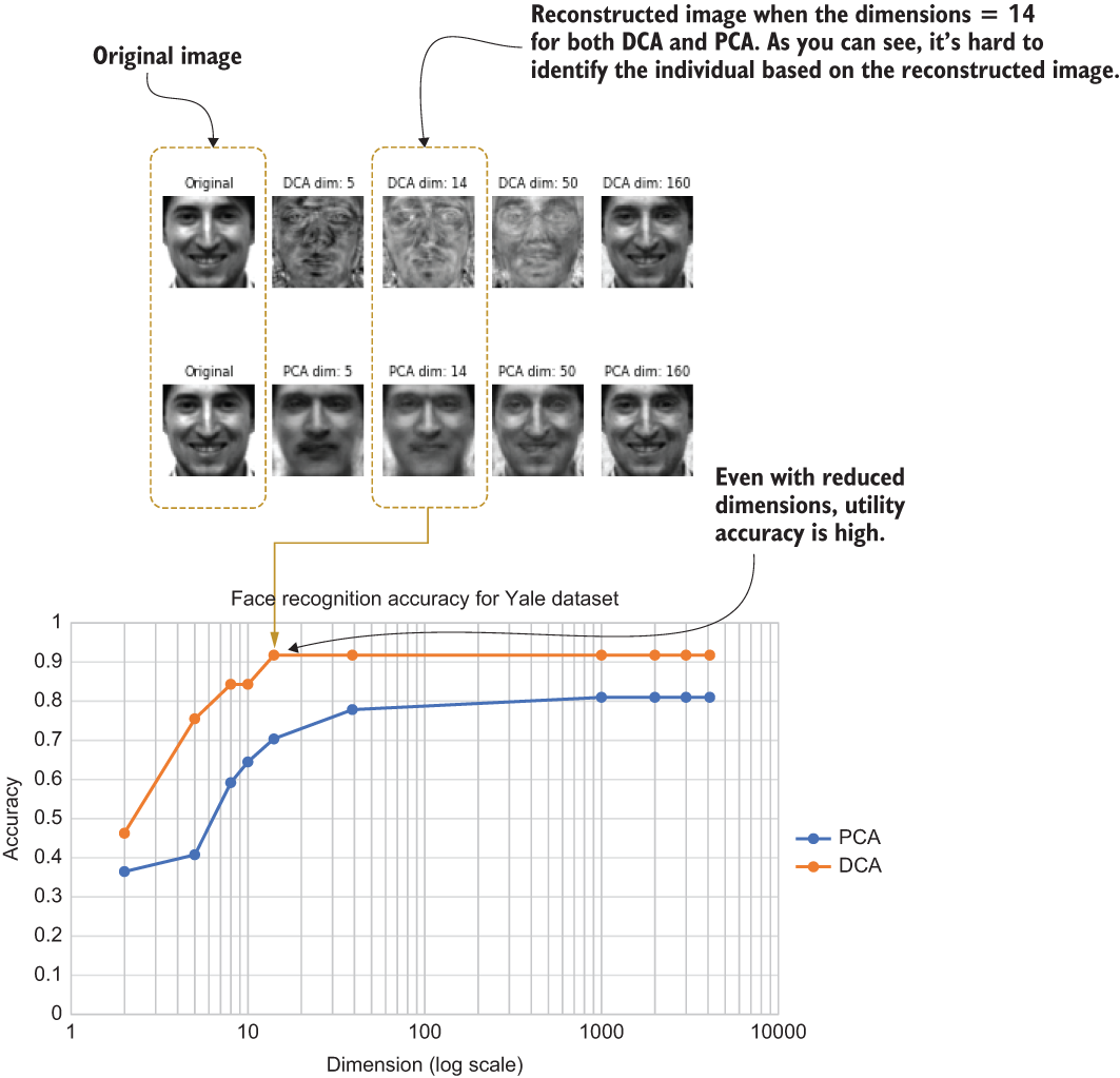
Figure 9.3 A comparison of the accuracy of the reconstructed images for different dimension settings

Now that we’ve investigated the accuracy of the utility, let’s see how hard it is for someone else to reconstruct the compressed image. This can be measured by the reconstruction error. To determine that, we need to go through the whole dataset, not just a couple of records. Thus we’ll modify the code a little bit, as shown in the following listing.

Listing 9.4 Calculating the average reconstruction error

import sys
sys.path.append('..');
import numpy as np
from discriminant_analysis import DCA, PCA
 
rho = 10; 
rho_p = -0.05;
 
dims = [2,5,8,10,14,39,1000,2000,3000,4096];
       
data_dir = './CompPrivacy/DataSet/Yale_Faces/';
X = np.loadtxt(data_dir+'Xyale.txt');
y = np.loadtxt(data_dir+'Yyale.txt');
           
reconErr_pca = np.zeros((len(dims)));
reconErr_dca = np.zeros((len(dims)));
 
mydca = DCA(rho,rho_p);
mypca = PCA();
mypca.fit(X);
mydca.fit(X,y);
 
D_pca = mypca.transform(X);                                            ❶
D_dca = mydca.transform(X); 
print('Principal and discriminant components were extracted.')
    
for j in range(len(dims)):
    Xrec = np.dot(D_pca[:,:dims[j]],mypca.components[:dims[j],:]);     ❷
    reconErr_pca[j] = sum(np.linalg.norm(X-Xrec,2,axis=1))/len(X);
    print('Average reconstruction error of %d-dimensional PCA: %f' 
              %(dims[j],reconErr_pca[j]));
        
    Xrec = mydca.inverse_transform(D_dca[:,:dims[j]],dim=dims[j]);     ❸
    reconErr_dca[j] = sum(np.linalg.norm(X-Xrec,2,axis=1))/len(X);
    print('Average reconstruction error of %d-dimensional DCA: %f' 
              %(dims[j],reconErr_dca[j]));
 
np.savetxt('reconErr_pca.out', reconErr_pca, delimiter=',')            ❹
np.savetxt('reconErr_dca.out', reconErr_dca, delimiter=',')

❶ Precompute all the components.

❷ Test the reconstruction error of PCA.

❸ Test the reconstruction error of DCA.

❹ Save the results to a text file.

Figure 9.4 shows the results of listing 9.4 plotted against different dimensions. As you can see, when the dimensions are lower, it is hard for someone to reconstruct the image accurately. For example, the DCA datapoint at dimension 14 has a very high value for the reconstruction error, making it very hard for someone to reconstruct the image. However, as you saw before, it still provides good accuracy for the face recognition task. This is the whole idea of using CP technologies for ML applications.

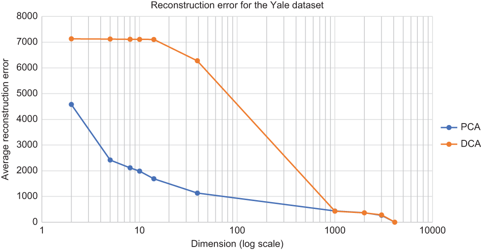
Figure 9.4 Comparing the average reconstruction error for different dimension settings

9.3.3 The effect of ρ' in DCA for privacy and utility

We have experimented with how dimension reduction can help determine privacy. When the number of dimensions is lower, more information is lost, yielding better privacy. But in DCA we have another parameter, ρ'. So far we have only changed the number of dimensions and kept ρ' as rho_p = -0.05. Now we will look at the importance of this parameter in determining the level of privacy by keeping the number of dimensions fixed.

The following listing is almost the same as listing 9.3, except that instead of going through several dimensions, now we’ll change the rho_p parameter to different values: [-0.05, -0.01, -0.001, 0.0, 0.001, 0.01, 0.05]. We’ll fix the dimensions at 160 (you can also try this with a different value).

Listing 9.5 Changing ρ' in DCA and determining the effect on privacy

import sys
sys.path.append('..');
import numpy as np
from discriminant_analysis import DCA
from matplotlib.pyplot import *
from random import randrange
 
def displayImage(vImage,height,width):
    mImage = np.reshape(vImage, (height,width)).T
    imshow(mImage, cmap='gray')
    axis('off')
    
height = 64
width = 64
 
rho = 10; 
rho_p = [-0.05,-0.01,-0.001,0.0,0.001,0.01,0.05]
selected_dim = 160
image_id = randrange(165)
       
data_dir = './CompPrivacy/DataSet/Yale_Faces/';
X = np.loadtxt(data_dir+'Xyale.txt');
y = np.loadtxt(data_dir+'Yyale.txt');
           
subplot(2,4,1)
title('Original',{'fontsize':8})
displayImage(X[image_id],height,width)
 
for j in range(len(rho_p)):    
    mydca = DCA(rho,rho_p[j]);   
    mydca.fit(X,y);
    D_dca = mydca.transform(X); 
    print('Discriminant components were extracted for rho_p: '+str(rho_p[j]))
    
    Xrec = mydca.inverse_transform(D_dca[:,:selected_dim],dim=selected_dim);
    eigV_dca = np.reshape(Xrec,(len(X),64,64))
    
    subplot(2,4,j+2)
    title('rho_p: ' + str(rho_p[j]),{'fontsize':8})
    displayImage(eigV_dca[image_id],height,width)
    
show()

The results are shown in figure 9.5. The top-left image is the original, and the rest of the images are produced with different rho_p values. As you can see, when the rho_p value changes from -0.05 to 0.05, the resultant image changes significantly, making it hard to identify. Thus, we can deduce that ρ' is also an important parameter in determining the level of privacy when DCA is used. As you can see, positive values of ρ' provide a much greater level of privacy than negative values.

Figure 9.5 Effect of ρ' on privacy with dimension fixed at 160 on the Yale dataset

We have now explored the possibility of integrating CP technologies into ML applications. You’ve seen that with a minimum number of dimensions, maximum face recognition accuracy is obtainable, and the privacy of the reconstructed image is still preserved. In the next section we’ll extend the discussion further with a case study on privacy preservation on horizontally partitioned data.

First, though, here are a few exercises you can explore to see the effect of ρ' on improving accuracy and to play with the different datasets.

Exercise 1

You now know that positive values of ρ' help to improve privacy. How about the accuracy of the face recognition task? Do positive values of ρ' help accuracy as well? Change the code in listing 9.3 and observe the utility accuracy and the average reconstruction error for each different ρ' value. (Hint: You can do this by adding another for loop that goes through the different rho_p values.)

Solution: In terms of the accuracy of the face recognition task, the value of ρ' has no significant effect. Try to plot ρ' against the accuracy, and you will see this clearly.

Exercise 2

All the experiments we have explored so far were based on the Yale dataset. Switch to the Olivetti dataset and rerun all the experiments to see whether the observations and patterns are similar. (Hint: This is quite straightforward. You just need to change the dataset name and the location.)

Solution: This solution is provided in the book’s source code repository.

Exercise 3

Now change the dataset to the glasses dataset. In this case, remember that the utility of the application will be identifying the person whether they wear a pair of glasses or not. The privacy target is still the reconstruction of the image. Change the code and see how PCA and DCA help here.

Solution: The solution is provided in the book’s source code repository.

9.4 Case study: Privacy-preserving PCA and DCA on horizontally partitioned data

As you already know, machine learning (ML) can be classified into two different categories or tasks: supervised tasks like regression and classification, and unsupervised tasks like clustering. In practice, these techniques are widely used in many different applications such as identity and access management, detecting fraudulent credit card transactions, building clinical decision support systems, and so on. These applications often use personal data, such as healthcare records, financial data, and the like, during the training and testing phases of ML.

While there are many different approaches, dimensionality reduction (DR) is an important ML tool that can be used to overcome different types of problems:

• Overfitting when the feature dimensions far exceed the number of training samples

• Performance degradation due to suboptimal search

• Higher computational costs and power consumption resulting from high dimensionality in the feature space

We’ve discussed a couple of DR methods in this chapter already: PCA and DCA.

As you’ll recall, PCA aims to project the data on the principal components with the highest variance, thus preserving most of the information while reducing the data dimensions. As you can see in figure 9.6 (a), most of the variability happens along with the first principal component (shown as PC-1). Hence, projecting all the points on that new axis could reduce the dimensions without sacrificing much data variability.

Compared to PCA, DCA is designed for supervised learning applications. The objective of DCA is not recoverability (for reducing the reconstruction error like PCA) but rather is improving the discriminant power of the learned classifiers so that they can effectively discriminate between different classes. Figure 9.6 (b) shows an example of a supervised learning problem where PCA would choose PC-1 as the principal component on which the data would be projected, because PC-1 is the direction of most variability. In contrast, DCA would choose PC-2, since it provides the highest discriminant power.

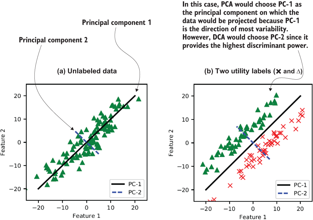
Figure 9.6 How dimensionality reduction works

Traditionally, PCA and DCA have been performed by gathering data in a centralized location, but in many applications (such as continuous authentication [5]), the data is distributed across multiple data owners. In such cases, collaborative learning is done on a joint dataset formed of samples held by different data owners, where each sample contains the same attributes (features). Such data is described as horizontally partitioned, since the data is represented as rows of similar features (columns), and each data owner holds a different set of rows in the joint data matrix.

In this situation, suppose a central entity (the data user) wants to compute a PCA (or DCA) projection matrix using the data distributed across multiple data owners in a privacy-preserving way. The data owners could then use the projection matrix to reduce the dimensions of their data. Such reduced dimensional data could then be used as the input to specific privacy-preserving ML algorithms that perform classification or regression.

In the case study in this section, we will be looking at the problem of a data user computing PCA and DCA projection matrices without compromising the privacy of the data owners. When it comes to distributed ML with PCA, privacy was not considered at all in early approaches. Later on, different privacy-preserving methods were proposed for PCA [6], but when it came to the implementation, they required all the data owners to remain online throughout the execution of the protocol, which was not very practical. In this case study, we’ll provide a solution to this problem by proposing and implementing a practical DR method using PCA and DCA in a privacy-preserving way.

In contrast to earlier approaches, the protocol that we are about to explore does not reveal any intermediate results (such as scatter matrices) and does not require data owners to interact with each other or remain online after submitting their individual encrypted shares. This newer approach can be utilized as a privacy-preserving data preprocessing stage before applying other privacy-preserving ML algorithms for classification or regression. Thus, it ensures both privacy and utility while applying ML algorithms to private data.

9.4.1 Achieving privacy preservation on horizontally partitioned data

Before we get into the details, let’s quickly walk through the key things that we’ll look at in this case study. Computing projection matrices to facilitate distributed privacy-preserving PCA (or DCA) requires computing the scatter matrices in a distributed fashion. We will use additive homomorphic encryption to compute the scatter matrices.

In addition to the data owners (who hold the data) and the data user (who aims to compute the projection matrix), we will assume the existence of a third entity, a crypto service provider (CSP), that will not collude with the data user. When data owners send the data, they need to compute their individual shares, encrypt them using homomorphic encryption with the CSP’s public key, and, finally, send these shares to the data user, who will aggregate these shares. After that, the CSP can build a garbled circuit that performs Eigen-decomposition on the scatter matrices computed from the aggregated shares (see the sidebar for a discussion of garbled circuits). Neither the data user nor the CSP can see the aggregated shares in their cleartext form, so data exchange protocols in this solution do not reveal any intermediate values, such as the user shares or scatter matrices. Moreover, this approach does not burden data owners with interacting with other data owners, and it does not require them to remain online after sending their encrypted shares, making these protocols practical.

9.4.2 Recapping dimensionality reduction approaches

Later in this chapter we’ll use the dimensionality reduction (DR) techniques that we discussed earlier and other privacy-enhancing techniques to achieve privacy preservation for PCA and DCA. Let’s quickly recap the DR methods that we discussed.

PCA is a DR method that is often used to reduce the dimensionality of large datasets. The idea is to transform a large set of variables into a smaller set in a way that still contains most of the information in the large set. Reducing the number of variables in a dataset naturally comes at the expense of accuracy. However, DR techniques trade a little accuracy for the simplicity of the approach. Since smaller datasets are easier to explore and visualize, and because they make analyzing data much easier and faster for ML algorithms, these DR techniques play a vital role.

While PCA is an unsupervised DR technique (it does not utilize data labels), DCA is a supervised method of DR. DCA selects a projection hyperplane that can effectively discriminate between different classes. At a high level, the key difference between these two techniques is that PCA assumes a linear relationship to the gradients, while DCA assumes a unimodal relationship.

In addition to PCA and DCA, many other DR techniques rely on two different steps discussed at the beginning of this chapter: computing a scatter matrix and computing eigenvalues. In general, these DR methods can be distinguished in terms of which scatter matrices are needed and which eigenvalue problems need to be solved. For instance, linear discriminant analysis (LDA) is a method similar to DCA (both are utility driven). We will not be going into the details here, but the main difference is that LDA solves eigenvalues utilizing a within-class scatter matrix, whereas DCA uses a between-class scatter matrix.

While DCA and LDA are utility-driven DR techniques, another class of DR approaches concentrates on utility-privacy optimization problems such as the multiclass discriminant ratio (MDR) [4]. We looked into the details of MDR at the beginning of this chapter. At a high level, MDR aims to maximize the separability of the utility classification problem (the intended task), while minimizing the separability of the privacy-sensitive classification problem (the sensitive task). It assumes that each data sample has two labels: a utility label (for the intended purpose of the data) and a privacy label (for specifying the type of sensitive information). Hence, we can obtain two between-class scatter matrices: one that is based on the utility labels and a second that is computed using the privacy labels.

9.4.3 Using additive homomorphic encryption

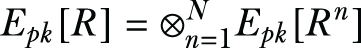
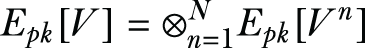
To facilitate the crypto service provider’s (CSP’s) function, additive homomorphic encryption will be an essential building block in our protocols. In section 3.4.1 we discussed homomorphic encryption. As you know, there are multiple semantically secure additive homomorphic encryption schemes. We will look at how the Paillier cryptosystem [7] can be used as an example of such encryption schemes. Let’s say function E_pk[∙] is an encryption operation indexed by a public key pk, and suppose D_sk[∙] is a decryption operation indexed by a secret key sk. The additive homomorphic encryption can be represented as E_pk [a + b] = E_pk[a] ⊗ E_pk [b], where ⊗ is the modulo multiplication operator in the encrypted domain. In addition, scalar multiplication can be achieved by E_pk[a]^b = E_pk[a ∙ b]. If you are interested in more details of the Paillier cryptosystem, you can refer to the original paper. You’ll need to understand the basic functionality of the homomorphic encryption scheme because we’ll use it in the next section.

Such encryption schemes only accept integers as plain text, but in most use cases, you’ll be dealing with real values when you are implementing ML applications. When dealing with ML, the typical approach is to discretize the data (the feature values) to obtain integer values.

9.4.4 Overview of the proposed approach

In this study, we’ll consider the case of horizontally partitioned data across multiple data owners. The system architecture is shown in figure 9.7. Suppose there are N data owners where each data owner n holds a set of feature vectors Xiⁱ ∈ ℝ^k×M with M number of features (dimensions) and i = 1, ..., k. Here, k is the total number of feature vectors. Thus, each data owner n will have a data matrix such that Xⁿ ∈ ℝ^k×M. In addition, in supervised learning, each sample x has a label y indicating that it belongs to one of the classes.

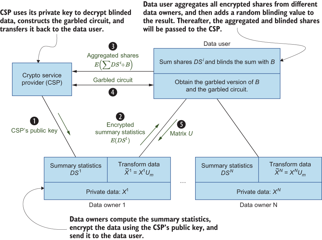
Figure 9.7 The system architecture and how it works

In this system, data users want to utilize the data and compute the PCA (or DCA) projection matrix from the data, which is horizontally partitioned among multiple data owners. There are many practical applications that fall under this data-sharing model. For example, with continuous authentication (CA) applications, a CA server needs to build authentication profiles for a group of registered users using ML algorithms, including DR techniques like PCA. Hence, the CA server (the data user) would need to compute PCA (or DCA) projection matrices using data that’s distributed (horizontally) across all registered users (the data owners).

We will look into the details of each step later, but let’s say there are two data owners, Alice and Bob, who would like to share their private data for a collaborative ML task. In this case, the ML task will be the data user. From a privacy standpoint, the most important concern is that any computation party, such as a data user or CSP, should not learn any of Alice’s or Bob’s input data or any intermediate values in cleartext format. That’s why we need to encrypt the data first. But when the data is encrypted, how can the ML algorithm learn anything? That’s where the homomorphic properties come into play, allowing you to still perform some calculations, like addition or subtraction, even with encrypted data.

Traditionally, PCA and DCA were only used in a centralized location on joint datasets (formed of data contributed by multiple data owners), but computing the projection matrix U requires the data owners to reveal their data. In this case study, we will modify the computation of the projection matrix to make it distributed and privacy-preserving. To facilitate this privacy-preserving computation, we’ll utilize a third party (the crypto service provider), which will engage in a relatively short one-round information exchange with the data user to compute the projection matrix. The data owners can then use the projection matrix to reduce the dimensions of their data. This reduced dimensional data can later be used as input to certain privacy-preserving ML algorithms that perform classification or regression.

When designing a security architecture, it is important to identify the threats that could be potentially harmful or vulnerable to the solution we are developing. Therefore, let’s quickly review the types of threats that we may face, so we can mitigate them in our solution. The main privacy requirement of our protocols is enabling data owners to preserve the privacy of their data. We’ll consider the adversaries to be the computation parties: the data user and the crypto service provider (CSP). Neither of these parties should have access to any of the data owner’s input data or any intermediate values (such as data owner shares or scatter matrices) in cleartext format. The data user should only learn the output of the PCA or DCA projection matrix and the eigenvalues.

The CSP’s primary role is to facilitate the scatter matrices’ privacy-preserving computation. To do that, the CSP is assumed to be an independent party, not colluding with the data user. For instance, the data user and the CSP could be different corporations that would not collude, if only to maintain their reputation and customer base. In addition, we’ll assume all participants are honest but curious (this is the semi-honest adversarial model). This means that all parties will correctly follow the protocol specification, but they could be curious and try to use the protocol transcripts to extract new information. Hence, both the data user and the CSP are considered semi-honest, non-colluding, but otherwise untrusted servers. We will also discuss extensions that could account for a data user colluding with a subset of the data owners to glean private information pertaining to a single data owner.

All communication between the data owners, the data user, and the CSP are assumed to be carried out on secure channels using well-known methods like SSL/TLS, digital certificates, and signatures.

9.4.5 How privacy-preserving computation works

Now that we’ve covered all the necessary background information, let’s proceed with the privacy-preserving computation of the scatter matrices and the PCA or DCA projection matrix. We’ll suppose that N data owners are willing to cooperate with a certain data user to compute the scatter matrices.

Privacy-preserving pca

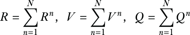
The first step in PCA is to compute the total scatter matrix in a distributed way. Let’s say the total scatter matrix is and that it can be computed in an iterative fashion. We have N data owners, and each data owner n carries a set of training samples, which we’ll denote as Pⁿ. Each data owner computes a set of values, which we’ll call local shares, as shown in the following equations:

The total scatter matrix can be found by summing the partial contributions from each party as follows,

where

It is important that the data owners should not send their local shares to the data user in cleartext, since they include statistical summaries of their data. The local shares can be encrypted using an additively homomorphic encryption scheme (such as Paillier’s cryptosystem) where the CSP provides the public key.

Upon receiving these encrypted shares, the data user can aggregate them to compute the encrypted intermediate values (namely R, V, and Q) and send them to the CSP for decryption after blinding the values. The data user can then use these aggregate values to compute the scatter matrix and the PCA projection matrix by using garbled circuits and oblivious transfer. Here, the blinding refers to adding random numbers to the encrypted values to prevent the CSP from learning anything about the data even in its aggregated form. (The values are blinded using an equivalent of a one-time pad.)

Let’s look at how this protocol works step by step to ensure privacy while preserving PCA:

1. Setting up the users—During setup, the CSP sends its public key pk for Paillier’s cryptosystem to the data owners and the data user based on their requests. This step could also include the official registration of the data owners with the CSP.

2. Computing local shares—Each data owner n will compute its own share DSⁿ = {Rⁿ, Vⁿ, Qⁿ} using the equations we discussed earlier. After discretizing all the values to obtain integer values, the data owners will encrypt Rⁿ, Vⁿ, and Qⁿ using the CSP’s public key to obtain E_pk[DSⁿ] = {E_pk[Rⁿ], E_pk[Vⁿ], E_pk[Qⁿ]}. Finally, each data owner sends E_pk[DSⁿ] to the data user.

3. Aggregating the local shares—The data user receives E_pk[DSⁿ] = {E_pk[Rⁿ], E_pk[Vⁿ], E_pk[Qⁿ]} from each data owner and proceeds to compute the encryption of R, V, and Q. More explicitly, the data user is capable of computing E_pk[R], E_pk[V], and E_pk[Q] from the encrypted data owner shares as follows:

   

   

   

   The data user adds some random integers to these aggregated values to mask them from the CSP, thus obtaining the blinded aggregated shares E_pk[R'], E_pk[V'], and E_pk[Q'], which can be sent to the CSP for decryption.

4. Using garbled circuits for eigenvalue decomposition (EVD):

   1. Once the blinded aggregated shares are received from the data user, the CSP will use its private key to decrypt them, E_pk[R'], E_pk[V'], and E_pk[Q']. Since CSP does not know the random values added by the data user, the CSP cannot learn the original aggregated values.

   2. The CSP will then construct a garbled circuit to perform EVD on the scatter matrix computed from the aggregated shares. The input to this garbled circuit is the garbled version of the blinded aggregate shares that the CSP decrypted and the blinding values which are generated and held by the data user.

   3. Since the CSP constructs the garbled circuit, it can obtain the garbled version of its input by itself. However, the data user needs to interact with the CSP using the oblivious transfer to obtain the garbled version of its input: the blinding values. Using oblivious transfer, we can guarantee that the CSP will not learn the blinding values held by the data user.

   4. The garbled circuit constructed by the CSP takes the two garbled inputs and computes the scatter matrix from the shares R', V', and Q' after subtracting the data user’s blinding values added in the previous steps. The CSP follows that by performing Eigen-decomposition on the scatter matrix to obtain the PCA projection matrix.

   5. The data user will receive the garbled circuit as its evaluator. This garbled circuit already has the CSP’s garbled input (decrypted and blinded aggregate shares), and the data user obtains the garbled version of the blinding values using oblivious transfer.

   6. Finally, the data user executes the garbled circuit and obtains the projection matrix and eigenvalues as output.

That is how privacy-preserving PCA can be implemented and computed in practical applications. We will look at the efficiency of this method later in the chapter. Now let’s look at how privacy-preserving DCA works.

Privacy-preserving dca

As we discussed in section 9.2, DCA computation requires the computation of the total scatter matrix and the signal matrix S_B. Furthermore, some other DCA formulations also use something called the noise matrix S_W. We will first quickly outline the distributed computation of S_B and S_W, and then we’ll move on to the protocol implementation details.

The computation of S_B and S_W could be different depending on whether the data owner has data that belongs to a single class or multiple classes. For instance, consider a spam email detection application where each data owner has spam and non-spam emails. This case represents two classes (spam and non-spam), and it is an example of a multiple-class data owner (MCDO). On the other hand, sometimes each data owner represents one class, as in continuous authentication systems. In this case, all their data would have the same label. This is an example of a single-class data owner (SCDO).

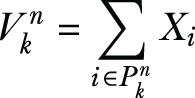
We will first review the equations for computing the scatter matrices S_B and S_W in a distributed way, and then we’ll present the protocol that performs the DCA computation in a privacy-preserving way. Let’s say each sample X_i has a label y_i indicating it belongs to one of the K classes C₁, C₂, ... , C_k. We’ll let μ denote the mean vector of the training samples in class C_k, and M_k denote the number of samples in class C_k. With that, the noise matrix S_W can be calculated as follows,

where the matrix O_k represents the share that pertains to class k. Since each data owner n maps to a single class k (in the SCDO case), we can write O_k = Oⁿ and have .

As for the case of multiple-class data owners (MCDO), each data owner n will hold data belonging to different classes. We’ll denote Pⁿ_k as the set of training samples held by data owner n that belong to class k. For each class k, a data owner can locally compute

In addition, Mⁿ_k can be computed as Mⁿ_k = |Pⁿ_k|, and the data owner would also compute the Rⁿ similar to PCA, as it is not restricted to a certain class. Now the S_W can be arranged as follows in terms of the partial contributions from data owners,

where

Now let’s look at how we can compute the signal matrix S_B. Both the single class (SCDO) and multiple classes (MCDO) are computed similarly. Moreover, the signal matrix can be computed directly from the aggregate data (V_k, M_k, V, M) described in previous equations as follows:

Unlike the scatter matrix, both the noise and signal matrices use class mean values in their computations. This will require the data owners to send per-class shares to the data user. If a data owner only sends the shares related to the classes the data owner has, this will leak knowledge of which classes belong to which data owner. Hence, it is recommended that all data owners send shares representing all classes, and when a data owner does not own certain class data, they can set that class share to all zeros.

Let’s look at how the privacy-preserving DCA protocol works step by step:

1. Setting up the users—This step is very similar to what we did for PCA. The CSP sends its public key pk for Paillier’s cryptosystem to the data owners and the data user based on their requests.

2. Computing local shares—Each data owner n computes Rⁿ from its data, and for each class labeled k, the data owner computes Vⁿ_k and Mⁿ_k. As noted earlier, if a data owner does not have samples pertaining to class k, they still generate Vⁿ_k and Mⁿ_k but set them to zeros. After discretization and obtaining integer values, the data owner will encrypt Rⁿ using the CSP’s public key to obtain E_pk[Rⁿ], and will also encrypt the class-based shares (Vⁿ_k and Mⁿ_k) to obtain {k, E_pk[Vⁿ_k], E_pk[Mⁿ_k]} for each class k. Finally, the data owner will send their own encrypted share DS n to the data user.

3. Aggregating the local shares—From each data owner, the data user receives DSⁿ, which includes E_pk[Rⁿ], and for each class k, it also includes {k, E_pk[Vⁿ_k], E_pk[Mⁿ_k]}. The data user then proceeds to reconstruct the encryption of R, the values of V_k , and the values of M_k as follows:

   

   And for each class k ∈ 1, ..., K, the data user computes

   

   

   Thereafter, the data user adds some random integers to these aggregated values to mask them from the CSP, thus obtaining the blinded shares E_pk[R'] in addition to the values of E_pk and E_pk. These blinded values are then sent to the CSP.

4. Performing the generalized eigenvalue decomposition (GEVD):

   1. The CSP will use its private key to decrypt the blinded shares E_pk[R'] and the values of E_pk[V’_k] and E_pk[M’_k] received from the data user. Without knowing the random values that were added by the data user, the CSP cannot learn the aggregated values.

   2. The CSP will then construct a garbled circuit to perform GEVD on the signal and the total scatter matrices computed from the aggregated shares. The input to this garbled circuit is the garbled version of the blinded aggregate shares that the CSP decrypted and the blinding values that were generated and held by the data user.

   3. As we discussed in the PCA case, since the CSP constructs the garbled circuit, it can obtain the garbled version of its input by itself. However, the data user needs to interact with the CSP using the oblivious transfer to obtain the garbled version of its input: the blinding values. This oblivious transfer guarantees that the CSP will not learn the blinding values held by the data user.

   4. The garbled circuit constructed by the CSP takes the two garbled inputs and removes the blinding values from the aggregated shares and uses the shares V'_k and M'_k to compute V and M. It then computes the total scatter matrix , and the signal matrix S_B, Finally, it performs the generalized eigenvalue decomposition to compute the DCA projection matrix.

   5. The data user will receive the garbled circuit as its evaluator. We know that this garbled circuit already has the CSP’s garbled input (decrypted and blinded aggregate shares), so they obtain the garbled version of the blinding values using oblivious transfer.

   6. Finally, the data user executes the garbled circuit and obtains the projection matrix and eigenvalues as output.

This is how privacy-preserving DCA can be implemented in your applications and use cases.

You have now gone through the equations showing how to transform data using encrypted shares and how to execute eigenvalue decomposition to work with PCA and DCA in meaningful ML tasks while preserving privacy. In the next section we will evaluate the efficiency and accuracy of these different approaches.

9.4.6 Evaluating the efficiency and accuracy of the privacy-preserving PCA and DCA

So far in this chapter, we’ve discussed the theoretical background and different methods of implementing CP (particularly PCA and DCA) in real-world ML applications. Here we’ll evaluate efficiency and accuracy of the implementations discussed in the previous sections of this case study (particularly in section 9.4.4). As we already discussed, when we integrate privacy into our ML tasks, it is important to maintain a balance between privacy and utility. Thus, we’ll evaluate this to see how effective the proposed approaches are for practical ML applications.

In this case study, the datasets we used for the experiments are from the UCI machine learning repository [8]. While PCA and DCA work for any type of ML algorithm, we chose classification, since the number of datasets available for classification, which was 255, far outnumbered those available for clustering or regression (around 55 each). Moreover, as the efficiency of the proposed protocols depends on the data dimensions (the number of features), we chose datasets with varying numbers of features: 8-50. Tables 9.1 and 9.2 summarize the number of features and classes for each dataset. The SVM is used as the classification task for these evaluations, and the number of data owners is set to 10 in all cases.

Analyzing the efficiency

Tables 9.1 and 9.2 show the timing data for performing privacy-preserving PCA and DCA on different datasets using Paillier’s key length of 1,024 bits. You can try this with different key sizes to see how it will affect the performance—you’ll find that when the key length is longer, performance is affected adversely.

The average time cost for the data owner refers to the total time it took the data owner to compute the individual shares and encrypt them. The average time cost for data users represents the time needed to collect each share from each data owner and add it to the current sum of these shares (in the encrypted domain).

The tables also show the time it took the CSP to decrypt the blinded aggregated values received from the data user. Finally, they show the time needed to run the eigenvalue decomposition using garbled circuits to compute the PCA or DCA projection matrices. The values in brackets refer to the number of principal components generated using the garbled circuit. Naturally, reducing this number would decrease the computation time for a given dataset. As we will be discussing in the next section, even 15 principal components for the SensIT Vehicle (Acoustic) dataset is enough to achieve adequate accuracy.

Finally, you’ll notice that increasing the dimension of the data will increase the computation time for all stages of the protocols, especially the eigenvalue decomposition.

Table 9.1 Efficiency of the distributed PCA

Table 9.2 Efficiency of the distributed DCA

Analyzing the accuracy of the ml task

Figure 9.8 and table 9.3 summarize the results of performing experiments to test the accuracy of the classification tasks after using our privacy-preserving protocols compared to results obtained using the Python library NumPy.

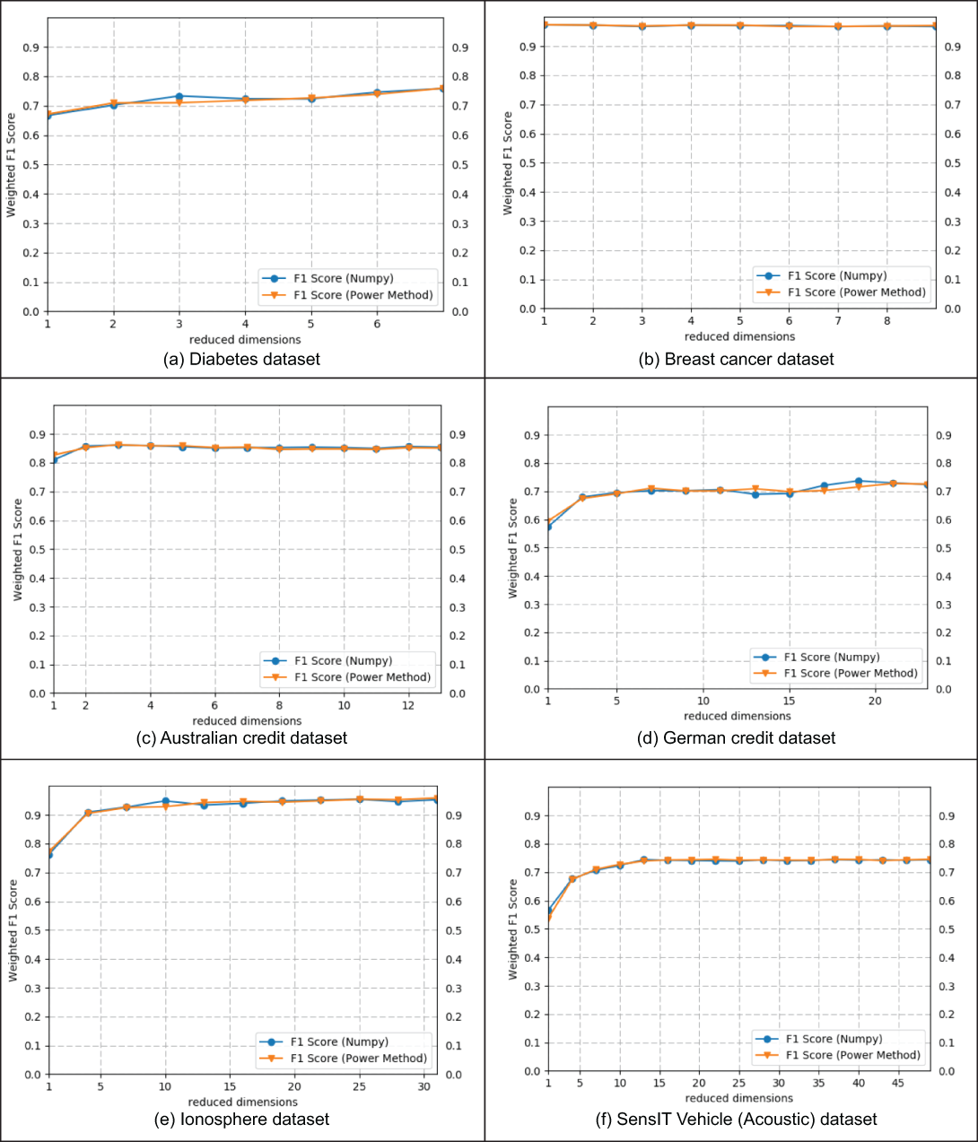
Figure 9.8 Privacy-preserving PCA accuracy

Here we are using the weighted F1 score to test the accuracy of the classifiers. The F1 score can be thought of as a weighted average of the precision and recall scores; a classifier is at its best when its F1 score is 1 and at its worst when the score is 0. The F1 score is one of the primary metrics utilized in ML applications to compare the performance of two classifiers. For more on how the F1 score works, refer back to section 3.4.3.

As a reminder, here is how you can calculate the F1 score:

The DCA results are shown in table 9.3 with one value each, since DCA projects the data to K - 1 dimensions (where K is the number of class labels), whereas PCA projects the data to a variable number of dimensions. As you can see, the protocols are correct and their results are equivalent to those obtained using NumPy. It should be noted that the slight fluctuation in the weighted F1 score is primarily due to the SVM parameter selection. However, the accuracy of both methods is almost the same.

Table 9.3 Privacy-preserving DCA accuracy

In this case study, we discussed how to implement privacy-preserving protocols for ML (particularly PCA and DCA) on horizontally partitioned data distributed across multiple data owners. From the results, it can be clearly seen that the approach is efficient, and it maintains the utility for data users while still preserving the privacy of the data owner’s data.

Summary

• The main problem with DP-based privacy preservation techniques is that they usually add excessive noise to the private data, resulting in a somewhat inevitable utility drop.

• Compressive privacy is an alternative approach (compared to DP) that can be utilized in many practical applications for privacy preservation without significant loss in the utility task.

• Compressive privacy essentially perturbs the data by projecting it to a lower-dimensional hyperplane via compression and DR techniques such that the data can be recovered without affecting the privacy.

• Different compressive privacy mechanisms serve different applications, but for machine learning and data mining tasks, PCA, DCA, and MDR are a few popular approaches.

• Compressive privacy technologies like PCA and DCA can also be used in the distributed setting to implement privacy-preserving protocols for machine learning.