• comparing the distributions of key variables between the modeling data set and the target population to verify that the sample adequately represents the target population

• defining sampling weights if necessary

• performing data-cleaning tasks that need to be done prior to launching SAS Enterprise Miner

Alternative strategies for developing predictive models using SAS Enterprise Miner are discussed at the end of this chapter.

1.2 Measurement Scales for Variables

Because many of the steps above involve a discussion of the data and types of variables in our data sets, I will first define the measurement scales for variables that are used in this book. In general, I have tried to follow the definitions given by Alan Agresti

• A categorical variable is one for which the measurement scale consists of a set of categories.

• Categorical variables for which levels (categories) do not have a natural ordering are called nominal.

• Categorical variables that do have a natural ordering of their levels are called ordinal.

• An interval variable is one that has numerical distances between any two levels of the scale.¹

According to the above definitions, the variables INCOME and AGE in Tables 1.1 to 1.5 and BAL_AFTER in Table 1.3 are interval-scaled variables. Because the variable RESP in Table 1.1 is categorical and has only two levels, it is called a binary variable. The variable LOSSFRQ in Table 1.2 is ordinal. (In SAS Enterprise Miner you can change its measurement scale to interval, but I have left it as ordinal.) The variables PRIORPR and NEXTPR in Table 1.5 are nominal.

Interval-scaled variables are sometimes called continuous. Continuous variables are treated as interval variables. Therefore I use the terms interval-scaled and continuous interchangeably.

I also use the terms ordered polychotomous variables and ordinal variables interchangeably. Similarly, I use the terms unordered polychotomous variables and nominal variables interchangeably.

1.3 Defining the Target

The first step in any data mining project is to define and measure the target variable to be predicted by the model that emerges from your analysis of the data. This section presents examples of this step applied to five different business questions.

1.3.1 Predicting Response to Direct Mail

In this example, a hypothetical auto insurance company wants to acquire customers through direct mail. The company wants to minimize mailing costs by targeting only the most responsive customers. Therefore, the company decides to use a response model. The target variable for this model is RESP, and it is binary, taking the value of 1 for response and 0 for no response.

Table 1.1 shows a simplified version of a data set used for modeling the binary target response (RESP).

Table 1.1

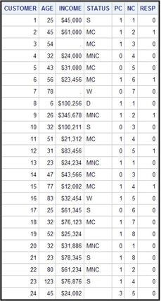
In Table 1.1 the variables AGE, INCOME, STATUS, PC, and NC are input variables (or explanatory variables). AGE and INCOME are numeric and, although they could theoretically be considered continuous, it is simply more practical to treat them as interval-scaled variables.

The variable STATUS is categorical and nominal-scaled. The categories of this variable are S if the customer is single and never married, MC if married with children, MNC if married without children, W if widowed, and D if divorced.

The variable PC is numeric and binary. It indicates whether the customers own a personal computeror not, taking the value 1 if they do and 0 if not. The variable NC represents the number of credit cards the customers own. You can decide whether this variable is ordinal or interval scaled.

The target variable is RESP and takes the value 1 if the customer responded, for example, to a mailing campaign, and 0 otherwise. A binary target can be either numeric or character; I could have recorded a response as Y instead of 1, and a non- response as N instead of 0, with virtually no implications for the form of the final equation.

Note that there are some extreme values in the table. For example, one customer’s age is recorded as 6. This is obviously a recording error, and the age should be corrected to show the actual value, if possible. Income has missing values that are shown as dots, while the nominal variable STATUS has missing values that are represented by blanks. The Impute node of SAS Enterprise Miner can be used to impute such missing values. See Chapters 2, 6, and 7 for details.

1.3.2 Predicting Risk in the Auto Insurance Industry

The auto insurance company wants to examine its customer data and classify its customers into different risk groups. The objective is to align the premiums it is charging with the risk rates of its customers. If high-risk customers are charged low premiums, the loss ratios will be too high and the company will be driven out of business. If low-risk customers are charged disproportionately high rates, then the company will lose customers to its competitors. By accurately assessing the risk profiles of its customers, the company hopes to set customers’ insurance premiums at an optimum level consistent with risk. A risk model is needed to assign a risk score to each existing customer.

In a risk model, loss frequency can be used as the target variable. Loss frequency is calculated as the number of losses due to accidents per car-year, where car-year is equal to the time since the auto insurance policy went into effect, expressed in years, multiplied by the number of cars covered by the policy. Loss frequency can be treated as either a continuous (interval-scaled) variable or a discrete (ordinal) variable that classifies each customer’s losses into a limited number of bins. (See Chapters 5 and 7 for details about bins.) For purposes of illustration, I model loss frequency as a continuous variable in Chapter 4 and as a discrete ordinal variable in Chapters 5 and 7. The loss frequency considered here is the loss arising from an accident in which the customer was “at fault,” so it could also be referred to as “at-fault accident frequency”. I use loss frequency, claim frequency, and accident frequency interchangeably.

Table 1.2 shows what the modeling data set might look like for developing a model with loss frequency as an ordinal target.

Table 1.2

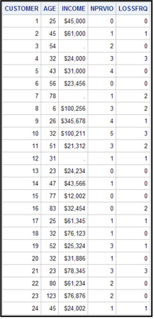
The target variable is LOSSFRQ, which represents the accidents per car-year incurred by a customer over a period of time. This variable is discussed in more detail in subsequent chapters in this book. For now it is sufficient to note that it is an ordinal variable that takes on values of 0, 1, 2, and 3. The input variables are AGE, INCOME, and NPRVIO. The variable NPRVIO represents the number of previous violations a customer had before he purchased the insurance policy.

1.3.3 Predicting Rate Sensitivity of Bank Deposit Products

In order to assess customers’ sensitivity to an increase in the interest rate on a savings account, a bank may conduct price tests. Suppose one such test involves offering a higher rate for a fixed period of time, called the promotion window.

In order to assess customer sensitivity to a rate increase, it is possible to fit three types of models to the data generated by the experiment:

• a response model to predict the probability of response

• a short-term demand model to predict the expected change in deposits during the promotion period

• a long-term demand model to predict the increase in the level of deposits beyond the promotion period

The target variable for the response model is binary: response or no response. The target variable for the short-term demand model is the increase in savings deposits during the promotion period net² of any concomitant declines in other accounts. The target variable for the long-term demand model is the amount of the increase remaining in customers’ bank accounts after the promotion period. In the case of this model, the promotion window for analysis has to be clearly defined, and only customer transactions that have occurred prior to the promotion window should be included as inputs in the modeling sample.

Table 1.3 shows what the data set looks like for modeling a continuous target.

Table 1.3

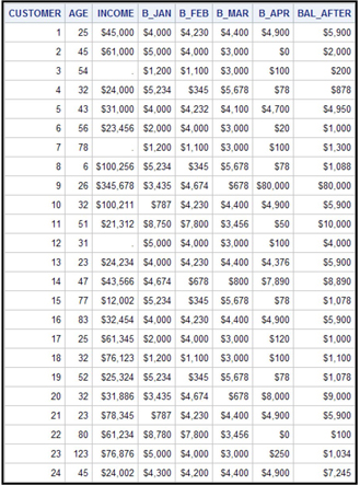
The data set shown in Table 1.3 represents an attempt by a hypothetical bank to induce its customers to increase their savings deposits by increasing the interest paid to them by a predetermined number of basis points. This increased interest rate was offered (let us assume) in May 2006. Customer deposits were then recorded at the end of May 2006 and stored in the data set shown in Table 1.3 under the variable name BAL_AFTER. The bank would like to know what type of customer is likely to increase her savings balances the most in response to a future incentive of the same amount. The target variable for this is the dollar amount of change in balances from a point before the promotion period to a point after the promotion period. The target variable is continuous. The inputs, or explanatory variables, are AGE, INCOME, B_JAN, B_FEB, B_MAR, and B_APR. The variables B_JAN, B_FEB, B_MAR, and B_APR refer to customers’ balances in all their accounts at the end of January, February, March, and April of 2006, respectively.

1.3.4 Predicting Customer Attrition

In banking, attrition may mean a customer closing a savings account, a checking account, or an investment account. In a model to predict attrition, the target variable can be either binary or continuous. For example, if a bank wants to identify customers who are likely to terminate their accounts at any time within a pre-defined interval of time in the future, it is possible to model attrition as a binary target. However, if the bank is interested in predicting the specific time at which the customer is likely to “attrit,” then it is better to model attrition as a continuous target—time to attrition.

In this example, attrition is modeled as a binary target. When you model attrition using a binary target, you must define a performance window during which you observe the occurrence or non-occurrence of the event. If a customer attrited during the performance window, the record shows 1 for the event and 0 otherwise.

Any customer transactions (deposits, withdrawals, and transfers of funds) that are used as inputs for developing the model should take place during the period prior to the performance window. The inputs window during which the transactions are observed, the performance window during which the event is observed, and the operational lag, which is the time delay in acquiring the inputs, are discussed in detail in Chapter 7 where an attrition model is developed.

Table 1.4 shows what the data set looks like for modeling customer attrition.

Table 1.4

In the data set shown in Table 1.4, the variable ATTR represents the customer attrition observed during the performance window, consisting of the months of June, July, and August of 2006. The target variable takes the value of 1 if a customer attrits during the performance window and 0 otherwise. Table1.4 shows the input variables for the model. They are AGE, INCOME, B_JAN, B_FEB, B_MAR, and B_APR. The variables B_JAN, B_FEB, B_MAR, and B_APR refer to customers’ balances for all of their accounts at the end of January, February, March, and April of 2006, respectively.

1.3.5 Predicting a Nominal Categorical (Unordered Polychotomous)Target

Assume that a hypothetical bank wants to predict, based on the products a customer currently owns and other characteristics, which product the customer is likely to purchase next. For example, a customer may currently have a savings account and a checking account, and the bank would like to know if the customer is likely to open an investment account or an IRA, or take out a mortgage. The target variable for this situation is nominal. Models with nominal targets are also used by market researchers who need to understand consumer preferences for different products or brands. Chapter 6 shows some examples of models with nominal targets.

Table 1.5 shows what a data set might look like for modeling a nominal categorical target.

Table 1.5

In Table 1.5, the input data includes the variable PRIORPR, which indicates the product or products owned by the customer of a hypothetical bank at the beginning of the performance window. The performance window, defined in the same way as in Section 1.3.4, is the time period during which a customer’s purchases are observed. Given that a customer owned certain products at the beginning of the performance window, we observe the next product that the customer purchased during the performance window and indicate it by the variable NEXTPR.

For each customer, the value for the variable PRIORPR indicates the product that was owned by the customer at the beginning of the performance window. The letter A might stand for a savings account, B might stand for a certificate of deposit, etc. Similarly, the value for the variable NEXTPR indicates the first product purchased by a customer during the performance window. For example, if the customer owned product B at the beginning of the performance window and purchased products X and Z, in that order, during the performance window, then the variable NEXTPR takes the value X. If the customer purchased Z and X, in that order, the variable NEXTPR takes the value Z, and the variable PRIORPR takes the value B on the customer’s record.

1.4 Sources of Modeling Data

There are two different scenarios by which data becomes available for modeling. For example, consider a marketing campaign. In the first scenario, the data is based on an experiment carried out by conducting a marketing campaign on a well-designed sample of customers drawn from the target population. In the second scenario, the data is a sample drawn from the results of a past marketing campaign and not from the target population. While the latter scenario is clearly less desirable, it is often necessary to make do with whatever data is available. In such cases, you can make some adjustments through observation weights to compensate for the lack of perfect compatibility between the modeling sample and the target population.

In either case, for modeling purposes, the file with the marketing campaign results is appended to data on customer characteristics and customer transactions. Although transaction data is not always available, these tend to be key drivers for predicting the attrition event.

1.4.1 Comparability between the Sample and Target Universe

Before launching a modeling project, you must verify that the sample is a good representation of the target universe. You can do this by comparing the distributions of some key variables in the sample and the target universe. For example, if the key characteristics are age and income, then you should compare the age and income distribution between the sample and the target universe.

1.4.2 Observation Weights

If the distributions of key characteristics in the sample and the target population are different, sometimes observation weights are used to correct for any bias. In order to detect the difference between the target population and the sample, you must have some prior knowledge of the target population. Assuming that age and income are the key characteristics, you can derive the weights as follows: Divide income into, let’s say, four groups and age into, say, three groups. Suppose that the target universe has N_ij people in the i^th age group and j^th income group, and assume that the sample has n_ij people in the same age-income group. In addition, suppose the total number of people in the target population is N, and the total number of people in the sample is n. In this case, the appropriate observation weight is (N_ij / N)/(n_ij / n) for the individual in the i^th age group and j^th income group in the sample. You should construct these observation weights and include them for each record in the modeling sample prior to launching SAS Enterprise Miner, in effect creating an additional variable in your data set. In SAS Enterprise Miner, you assign the role of Frequency to this variable in order for the modeling tools to consider these weights in estimating the models. This situation inevitably arises when you do not have a scientific sample drawn from the target population, which is very often the case.

However, another source of bias is often deliberately introduced. This bias is due to over-sampling of rare events. For example, in response modeling, if the response rate is very low, you must include all the responders available and only a random fraction of non-responders. The bias introduced by such over-sampling is corrected by adjusting the predicted probabilities with prior probabilities. These techniques are discussed in Section 4.8.2.

1.5 Pre-Processing the Data

Pre-processing has several purposes:

• eliminate obviously irrelevant data elements, e.g., name, social security number, street address, etc., that clearly have no effect on the target variable

• convert the data to an appropriate measurement scale, especially converting categorical (nominal scaled) data to interval scaled when appropriate

• eliminate variables with highly skewed distributions

• eliminate inputs which are really target variables disguised as inputs

• impute missing values

Although you can do many cleaning tasks within SAS Enterprise Miner, there are some that you should do prior to launching SAS Enterprise Miner.

1.5.1 Data Cleaning Before Launching SAS Enterprise Miner

Data vendors sometimes treat interval-scaled variables, such as birth date or income, as character variables. If a variable such as birth date is entered as a character variable, it is treated by SAS Enterprise Miner as a categorical variable with many categories. To avoid such a situation, it is better to derive a numeric variable from the character variable and then drop the original character variable from your data set.

Similarly, income is sometimes represented as a character variable. The character A may stand for $20K ($20,000), B for $30K, etc. To convert the income variable to an ordinal or interval scale, it is best to create a new version of the income variable in which all the values are numeric, and then eliminate the character version of income.

Another situation which requires data cleaning that cannot be done within SAS Enterprise Miner arises when the target variable is disguised as an input variable. For example, a financial institution wants to model customer attrition in its brokerage accounts. The model needs to predict the probability of attrition during a time interval of three months in the future. The institution decides to develop the model based on actual attrition during a performance window of three months. The objective is to predict attritions based on customers’ demographic and income profiles, and balance activity in their brokerage accounts prior to the window. The binary target variable takes the value of 1 if the customer attrits and 0 otherwise. If a customer’s balance in his brokerage account is 0 for two consecutive months, then he is considered an attritor, and the target value is set to 1. If the data set includes both the target variable (attrition/no attrition) and the balances during the performance window, then the account balances may be inadvertently treated as input variables. To prevent this, inputs which are really target variables disguised as input variables should be removed before launching SAS Enterprise Miner.

1.5.2 Data Cleaning After Launching SAS Enterprise Miner

Display 1.1 shows an example of a variable that is highly skewed. The variable is MS, which indicates the marital status of a customer. The variable RESP represents customer response to mail. It takes the value of 1 if a customer responds, and 0 otherwise. In this hypothetical sample, there are only 100 customers with marital status M (married), and 2900 with S (single). None of the married customers are responders. An unusual situation such as this may cause the marital status variable to play a much more significant role in the predictive model than is really warranted, because the model tends to infer that all the married customers were non-responders because they were married. The real reason there were no responders among them is simply that there were so few married customers in the sample.

Display 1.1

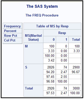
These kinds of variables can produce spurious results if used in the model. You can identify these variables using the StatExplore node, set their roles to Rejected in the Input Data node, and drop them from the table using the Drop node.

The Filter node can be used for eliminating observations with extreme values, although I do not recommend elimination of observations. Correcting them or capping them instead might be better, in order to avoid introducing any bias into the model parameters. The Impute node offers a variety of methods for imputing missing values. These nodes are discussed in the next chapter. Imputing missing values is necessary when you use Regression or Neural Network nodes.

1.6 Alternative Modeling Strategies

The choice of modeling strategy depends on the modeling tool and the number of inputs under consideration for modeling. Here are examples of two possible strategies when using the Regression node.

1.6.1 Regression with a Moderate Number of Input Variables

Pre-process the data:

• Eliminate obviously irrelevant variables.

• Convert nominal-scaled inputs with too many levels to numeric interval-scaled inputs, if appropriate.

• Create composite variables (such as average balance in a savings account during the six months prior to a promotion campaign) from the original variables if necessary. This can also be done with SAS Enterprise Miner using the SAS Code node.

Next, use SAS Enterprise Miner to perform these tasks:

• Impute missing values.

• Transform the input variables.

• Partition the modeling data set into train, validate, and test (when the available data is large enough) samples. Partitioning can be done prior to imputation and transformation, because SAS Enterprise Miner automatically applies these to all parts of the data.

• Run the Regression node with the Stepwise option.

1.6.2 Regression with a Large Number of Input Variables

Pre-process the data:

• Eliminate obviously irrelevant variables.

• Convert nominal-scaled inputs with too many levels to numeric interval-scaled inputs, if appropriate.

• Combine variables if necessary.

Next, use SAS Enterprise Miner to perform these tasks:

• Impute missing values.

• Make a preliminary variable selection. (Note: This step is not included in Section 1.6.1.)

• Group categorical variables (collapse levels).

• Transform interval-scaled inputs.

• Partition the data set into train, validate, and test samples.

• Run the Regression node with the Stepwise option.

The steps given in Sections 1.6.1 and 1.6.2 are only two of many possibilities. For example, one can use the Decision Tree node to make a variable selection and create dummy variables to then use in the Regression node.

1.7 Notes

1. Alan Agresti, Categorical Data Analysis (New York, NY: John Wiley & Sons, 1990), 2.

2. If a customer increased savings deposits by $100 but decreased checking deposits by $20, then the net increase is $80. Here, net means excluding.

..................Content has been hidden....................

You can't read the all page of ebook, please click here login for view all page.

Table of Contents for Chapter 1: Research Strategy

Create new playlist

Sign In

Sign Up

Chapter 1: Research Strategy

1.1 Introduction