6

Reliability Prediction and Modelling

6.1 Introduction

An accurate prediction of the reliability of a new product, before it is manufactured or marketed, is obviously highly desirable. Depending upon the product and its market, advance knowledge of reliability would allow accurate forecasts to be made of support costs, spares requirements, warranty costs, marketability, and so on. However, a reliability prediction can rarely be made with high accuracy or confidence. Nevertheless, even a tentative estimate can provide a basis for forecasting of dependent factors such as life cycle costs. Reliability prediction can also be valuable as part of the study and design processes, for comparing options and for highlighting critical reliability features of designs.

If a new engineered system is being planned, which will supersede an existing system, and the reliability of the existing system is known, then its reliability could reasonably be used as a starting point for predicting the likely reliability of the new system. However, the changes that will be introduced in the new system will be likely to affect its reliability: for example, more functions might be controlled through software, novel subsystems or components might be included, and so on. Some of these changes could enhance reliability, others might introduce new risks. There will also be programme and management aspects that would influence reliability, such as commitment and resources applied to achievement of quality and reliability objectives, testing strategies and constraints, in particular the time available for development. These aspects will be discussed in later chapters. This top-down approach can be applied to any new product or system. Even if there is no comparable product already in service, an estimate can and should be made, based on risks and commitment.

The prediction begins at the level of the overall system and as the system becomes more closely defined it can be extended to more detailed levels. Eventually, in principle, it is necessary to consider the reliability contributions of individual parts. However, the lower the level of analysis, the greater is the potential uncertainty inherent in predicting reliability of the whole system. It is important to remember that many system failures are not caused by failures of parts and not all part failures cause system failures.

The common approach to predicting reliability is to estimate the contributions of each part, and work upwards to the overall product or system level. The ‘parts count’ method (see later in this chapter) is widely used, but it is very dependent upon the availability of credible data. Databases providing failure rates at the part level have been developed and published, for electronic and non-electronic parts, which will be discussed later in this chapter. Since reliability is also affected strongly by factors such as knowledge and motivation of design and test engineers, the amount and quality of testing, action on failures discovered during test, quality of production, and, when applicable, maintenance skills, these factors must be taken into account as well. In many cases they can be much more significant than past data. Therefore reliability databases must always be treated with caution as a basis for predicting the reliability of new systems. There is no intrinsic limit to the reliability that can be achieved, but the database approach to prediction can imply that there is.

6.2 Fundamental Limitations of Reliability Prediction

In engineering and science we use mathematical models for prediction. For example, the power consumption of a new electronic system can be predicted using Ohm's law and the model power = current × emf. Likewise, we can predict future planetary positions using Newton's laws and our knowledge of the present positions, velocities and masses. These laws are valid within the appropriate domain (e.g. Ohm's law does not hold at temperatures near absolute zero; Newton's laws are not valid at the subatomic level). However, for practical, everyday purposes such deterministic laws serve our purposes well, and we use them to make predictions, taking due account of such practical aspects as measurement errors in initial conditions.

Whilst most laws in physics, for practical predictive purposes, can be considered to be deterministic, the underlying mechanisms can be stochastic. For example, the pressure exerted by a gas in an enclosure is a function of the random motions of very large numbers of molecules. The statistical central limiting theorem, applied to such a vast number of separate random events and interactions, enables us to use the average effect of the molecular kinetic energy to predict the value we call pressure. Thus Boyle's law is really empirical, as are other ‘deterministic’ physical laws such as Ohm's law. It is only at the level of individual or very few actions and interactions, such as in nuclear physics experiments, that physicists find it necessary to take account of uncertainty due to the stochastic nature of the underlying processes. However, for practical purposes we ignore the infinitesimal variations, particularly as they are often not even measurable, in the same way as we accept the Newtonian view.

For a mathematical model to be accepted as a basis for scientific prediction, it must be based upon a theory which explains the relationship. It is also necessary for the model to be based upon unambiguous definitions of the parameters used. Finally, scientists, and therefore engineers, expect the predictions made using the models to be always repeatable. If a model used in science is found not to predict correctly an outcome under certain circumstances this is taken as evidence that the model, and the underlying theory, needs to be revised, and a new theory is postulated.

The concept of deriving mathematical models which could be used to predict reliability, in the same way as models are developed and used in other scientific and engineering fields, is intuitively appealing, and has attracted much attention. Laws of physics are taken into account in some reliability prediction models; however there are many more factors causing parts to fail (some of them are unknown), therefore predictions in reliability typically have a higher degree of uncertainty. For example, failure rate models have been derived for electronic components, based upon parameters such as operating temperature and other stresses. These are described below and in Chapters 9 and 13. Similar models have been derived for non-electronic components, and even for computer software. Sometimes these models are as simple as a single fixed value for failure rate or reliability, or a fixed value with simple modifying factors. However, some of the models derived, particularly for electronic parts, are quite complex, taking account of many factors considered likely to affect reliability.

A model such as Ohm's law is credible because there is no question as to whether or not an electric current flows when an emf is applied across a conductor. However, whilst an engineering component might have properties such as conductance, mass, and so on, all unambiguously defined and measurable, it is very unlikely to have an intrinsic reliability that meets such criteria. For example, a good transistor or hydraulic actuator, if correctly applied, should not fail in use, during the expected life of the system in which it is used. If failures do occur in a population of these components in these systems, the causes, modes of failure and distributions of times to failure could be due to a range of different physical or chemical causes, as well as factors other than those explainable in purely physical or chemical terms. Some transistors might fail because of accidental overstress, some because of processing defects, or there may be no failures at all. If the hydraulic actuators are operated for a long time in a harsh environment, some might develop leaks which some operators might classify as failures. Also, failure, or the absence of failure, is heavily dependent upon human actions and perceptions. This is never true of laws of nature. This represents a fundamental limitation of the concept of reliability prediction using mathematical models.

As Niels Bohr, the famous Danish physicist once jokingly said ‘Prediction is very difficult – especially if it is about the future.’ We saw in Chapter 5 how reliability can vary by orders of magnitude with small changes in load and strength distributions, and the large amount of uncertainty inherent in estimating reliability from the load-strength model.

Another serious limitation arises from the fact that reliability models are usually based upon statistical analysis of past data. Much more data is required to derive a statistical relationship than to confirm a deterministic (theory-based) one, and even then there will be uncertainty because the sample can seldom be taken to be wholly representative of the whole population. For example, the true value of a life parameter is never known, only its distribution about an expected value, so we cannot say when failure will occur. Sometimes we can say that the likelihood increases, for example, in fatigue testing or if we detect wear in a bearing, but we can very rarely predict the time of failure. A statistically-derived relationship can never by itself be proof of a causal connection or even establish a theory. It must be supported by theory based upon an understanding of the cause-and-effect relationship.

Depending on the situation, a prediction can be based on past data, so long as we are sure that the underlying conditions which can affect future behaviour will not change significantly. However, since engineering is very much concerned with deliberate change, in design, processes and applications, predictions of reliability based solely on past data ignore the fact that changes might be made with the objective of improving reliability. Alternatively, sometimes changes introduce new reliability problems. Of course there are situations in which we can assume that change will not be significant, or in which we can extrapolate taking account of the likely effectiveness of planned changes. For example, in a system containing many parts which are subject to progressive deterioration, for example, an office lighting system containing many fluorescent lighting units, we can predict the frequency and pattern of failures fairly accurately, but these are special cases.

In general, it is important to appreciate that predictions of reliability can seldom be considered as better than rough estimates, and that achieved reliability can be considerably different to the predicted value.

6.3 Standards Based Reliability Prediction

Standards based reliability prediction is a methodology based on failure rate estimates published in globally recognized standards, both military and commercial. In some cases manufacturers are obliged by their customers or by contractual clauses to perform reliability prediction based on published standards.

A typical standards based reliability prediction treats devices as serial, meaning that one component failure causes a failure of a whole system. The other key assumption is a constant failure rate, which is modelled by the exponential distribution (see Section 2.6.3). This generally represents the useful life of a component where failures are considered random events (i.e. no wearout or early failures problem). It is well recognized in the engineering community that the assumption of a constant failure rate for both electronic and non-electronic parts can be misleading.

The most common approach is to state failure rates, expressed as failures per unit of time, often million (or even billion) hours. One failure per billion hours (10⁹ hours) is commonly referred as one FIT. However, since FIT stands for Failure in Time, this unit of failure rate measure has not been universally accepted in the reliability engineering community. For non-repairable items this may be interpreted as the failure rate contribution to the system failure rate. These data are then used to synthesize system failure rate, by summation and by taking account of system configuration, as described later. Summation of part failure rates is generally referred to as the ‘parts count’ method. Reliability data can be useful in specific prediction applications, such as aircraft, petrochemical plant, computers or automobiles, when the data are derived from the area of application. However, such data should not be transferred from one application area to another without careful assessment. Even within the application area they should be used with care, since even then conditions can vary widely. An electric motor used to perform the same function, under the same loading conditions as previously in a new design of photocopier, might be expected to show the same failure pattern. However, if the motor is to be used for a different function, with different operating cycles, or even if it is bought from a different supplier, the old failure data might not be appropriate.

The commonly used standards include MIL-HDBK-217, Bellcore/Telcordia (SR-332), NSWC-06/LE10, China 299B, RDF 2000 and several others discussed later in this chapter. The typical analysis methods used by these standards include parts count and parts stress analysis methods. The parts count method requires less information, typically part quantities, quality levels and application environment. It is most applicable during very early design or proposal phases of a project.

6.3.1 MIL-HDBK-217

Probably the best known source of failure rate data for electronic components is US MIL-HDBK-217 (1995). It utilizes most of the principles listed before and is based on generic failure rates for electronic components collected over the years by the US Military. This handbook uses two methods of reliability prediction – parts count and parts stress. The parts count method assumes average stress levels as a means of providing an early design estimate of the failure rates. The overall equipment failure rate (ReliaSoft, 2006) can be calculated as:

where: n = number of parts categories (e.g. electrolytic capacitor, inductor, etc.).

The π-factors vary for component types and categories.

The parts stress method requires the greatest degree of detailed information. It is applied in the later phases of design when actual hardware and circuits are being designed. The parts stress method takes into account more information and the failure rate equations for each part contain more π-factors reflecting product environment, electrical stress, temperature factor, application environment, and other information specific to a component type and category. For example, the predicted failure rate for microcircuits can be calculated as:

Where π_Q, π_E, π_T and π_L are quality, environmental, temperature and learning factors respectively. C₁ is a die complexity factor based upon the chip gate count, or bit count for memory devices, or transistor count for linear devices and C₂ is a complexity factor based upon packaging aspects (number of pins, package type, etc.).

The criticisms of MIL-HDBK-217, which apply to most other standards-based methods for electronics include the following:

1. Experience shows that only a proportion of failures of modern electronic systems are due to components failing owing to internal causes.
2. The temperature dependence of failure rate is not always supported by modern experience or by considerations of physics of failure.
3. Several other parameters used in the models are of doubtful validity. For example, it is not true that failure rate increases significantly with increasing complexity, as continual process improvements counteract the effects of complexity.
4. The models do not take account of many factors that do affect reliability, such as transient overstress, temperature cycling, variation, EMI/EMC and control of assembly, test and maintenance.

Despite its flaws and the fact that MIL-HDBK-217 has not been updated since 1994 it is still being used to predict reliability. Therefore, there have been some efforts led by the United States Naval Surface Warfare Center (NSWC) to release MIL-HBDK-217 Revision G which would significantly update the existing standard including the introduction of aspects of physics of failure into the prediction procedure (see McLeish, 2010).

6.3.2 Telcordia SR-332 (Formerly Bellcore)

Other data sources for electronic components have been produced and published by non-military organizations, such as telecommunications companies for commercial applications. One of the most commonly used standards (particularly in Europe) is Telcordia SR-332, which was an update of the Bellcore document TR-332, Issue 6. The Bellcore reliability prediction model was originally developed by AT&T Bell Labs and was based on equations from MIL-HDBK-217, modified to better represent telecommunications industry field experience.

Telcordia SR-332 uses three different methods. Method I allows the user to obtain only the generic failure rates that are proposed by the Bellcore/Telcordia prediction standard. Method II allows the user to combine lab test data with the generic failure rates given in the standard. Method III allows the user to combine field data with the generic failure rates given in the standard. Additionally, SR-332 stresses the early life (infant mortality) problems of electronics and the use of burn-in by manufacturers to reduce the severity of infant mortality by weeding out weak components that suffer from early life problems (see ReliaSoft (2006) for more details). SR-332 also applies a First-Year-Multiplier factor that accounts for infant mortality risks in the failure rate prediction. The standard also applies a ‘credit’ for the use of a burn-in period and reduces the First-Year-Multiplier accordingly (i.e. the multiplier is smaller for longer periods of burn-in).

6.3.3 IEC 62380 (Formerly RDF 2000)

IEC Standard 62 380 TR Edition 1 was developed from RDF 2000, also formerly known as UTEC 80 810 (UTEC80810, 2000). This standard was designed as a further development of MIL-HDBK-217 where the multiplicative failure rate model was replaced by additive and multiplicative combinations of π-factors and failure rates. This standard allows specification of a temperature mission profile with different phases. The phases can have different temperatures that influence the failure rate of the components. The phases can also be of different types (on/off, permanently on, dormant) with various average outside temperature swings seen by the equipment. Those phases affect the failure rate calculation in different ways, as they apply different stresses on the components.

6.3.4 NSWC-06/LE10

Several databases have also been produced for non-electronic components, such as NSWC-06, 2006. This standard was developed from its earlier NSWC-98 version and uses a series of models for various categories of mechanical components to predict failure rates, which are affected by temperature, stresses, flow rates and various other parameters. The categories of mechanical equipment include seals, gaskets, springs, solenoids, valve assemblies, bearings, gears and splines, actuators, pumps, filters, brakes, compressors, electric motors and other non-electronic parts.

Many of the categories of mechanical equipment are in fact composed of a collection of sub-components which must be modelled by the user. For example, a collection for an electric motor would include bearings, motor windings, brushes, armature shaft, housing, gears. The user should be familiar with the equipment and the Handbook so that the correct type and number of sub-components can be included in the model.

Critics of this method note that the variety of types and applications of mechanical parts covered in the NSWC standard is very diverse, which amplifies the uncertainty of this type of prediction. Also, there is no general unit of operating time for a gasket or a spring, as there might be for an electronic component.

6.3.5 PRISM and 217Plus

The PRISM¯ reliability prediction tool was released in early 2000 by then the Reliability Analysis Center (RAC) to overcome the limitations of MIL-HDBK-217, which was not being actively maintained or updated (for more details see Dylis and Priore, 2001 and Alion, 2011). Also, the perception was that MIL-HDBK-217 produced pessimistic results due to the combined effect of multiplied π-factors. The premise of traditional methods of reliability predictions, such as MIL-HDBK-217, is that the failure rate of a system is primarily based on the components comprising that system. RAC data identified that more than 78% of failures stem from non-component causes, namely: design deficiencies, manufacturing defects, poor system management techniques such as inadequate requirements, wearout, software, induced and no-defect-found failures. In response to this, the RAC developed PRISM for estimating the failure rate of electronic systems. The PRISM model development was based on large amounts of field and test data from both defense and commercial applications.

Instead of using the multiplicative modelling approach as used by MIL-HDBK-217, PRISM utilizes additive and multiplicative combinations of π-factors and failure rates λ for each class of failure mechanism. This approach is somewhat similar to the method of RDF 2000. PRISM incorporates new component reliability prediction models, includes a process for assessing the reliability of systems due to non-component variables, and includes a software reliability model. PRISM also allows the user to tailor the prediction based upon all available data including field data on a similar ‘predecessor’ system, and component-level test data. The PRISM-predicted failure rate model takes a form of:

where: n = number of parts categories.

For example, π_eλ_e-addend would represent the contribution of product failure rate and π-factor for environmental stresses, π_oλ_o for operational stresses, and so on.

217Plus™ is a spin-off of PRISM, which generally uses the same modelling methodology, but has increased the number of part type failure rate models. 217Plus™ models also include: connectors, switches, relays, inductors, transformers and opto-electronic devices. For more information see Nicholls, (2007).

6.3.6 China 299B (GJB/z 299B)

The GJB/z 299B Reliability Calculation Model for Electronic Equipment (often referred as China 299B) is a Chinese standard translated into English in 2001. This standard is a reliability prediction program based on the internationally recognized method of calculating electronic equipment reliability and was developed for the Chinese military. The standard is very similar to MIL-HDBK-217 and includes both parts count and parts stress analysis methods. This standard uses a series of models for various categories of electronic, electrical and electro-mechanical components to predict failure rates that are affected by environmental conditions, quality levels, stress conditions and various other parameters. It provides the methodology of calculating failure rates at both component and system level.

6.3.7 Other Standards

The list of the standards mentioned in this section is non-exhaustive and does not include less commonly used reliability prediction standards, some of which have been discontinued, but still maintain a limited use.

The British Telecom Handbook of Reliability Data (see British Telecom, 1995) is quite similar in approach to MIL-HDBK-217. Other less common standards include Siemens reliability standard SN29500.1 and its updated version SN 29 500-2005-1 as well as ‘Italtel Reliability Prediction Handbook,’ published by Italtel in 1993 and Nippon's NTT procedure (Nippon, 1985) both discontinued.

The maintained standards include FIDES guide, updated in 2009 (FIDES, 2009). The FIDES methodology is based on the physics of failures and is supported by the analysis of test data, field returns and existing modelling. It is therefore different from the traditional methods developed mainly through statistical analysis of field returns. The methodology takes account of failures derived from development or manufacturing errors and overstresses (electrical, mechanical, thermal) related to the application.

Another non-electronic components standard is NPRD-95, ‘Non-electronic Parts Reliability Data’, released by RAC in the mid 1990-s. Part categories include actuators, batteries, pumps, and so on. Under the category the user would select a certain subtype (e.g. for batteries – Carbon Zinc, Lithium, etc.) in the same way as in NSWC-06.

6.3.8 IEEE Standard 1413

IEEE Standard 1413 (2003) has been created to establish a framework around which reliability prediction should be performed for electronic systems, though it could be applied to any technology. Prediction results obtained from an IEEE 1413 compliant reliability prediction are accompanied by responses to a set of questions identified in the standard. It identifies required elements for an understandable and credible reliability prediction with information to evaluate the effective use of the prediction results. IEEE 1413 however does not provide instructions for how to perform reliability prediction and does not judge any of the methodologies. In particular, an IEEE 1413 compliant prediction provides documentation of:

• the prediction results,
• the intended use of prediction results,
• the method(s) used,
• inputs required for selected method(s),
• the extent to which each input is known,
• – the source of known input data,
• assumptions for unknown input data,
• figures of merit,
• confidence in prediction,
• sources of uncertainty,
• limitations and
• repeatability.

6.3.9 Software Tools for Reliability Prediction

Calculating reliability prediction by hand, especially for a system with a large number of parts, is obviously a long and tedious procedure prone to errors. There is a variety of commercial software packages available to a practitioner to run the reliability prediction based on a bill of materials (BOM), operational environments, applications, component stress data, and other information available during a system design phase. Most software packages allow a user to choose between the reliability prediction standards or run them in parallel. A non-exhaustive list of reliability prediction packages includes Lambda Predict¯ by ReliaSoft, CARE¯ by BQR, ITEM ToolKit, Reliability Workbench by Isograph, RAM COMMANDER by Reliass, and several others. Most of the software packages have capabilities of adding user-defined failure rates databases in addition to the published standards listed in this chapter.

6.4 Other Methods for Reliability Predictions

6.4.1 Field Return Based Methods

Some manufacturers prefer reliability predictions conducted with databases containing their own proprietary data. Failure rates can be calculated based on the field return, maintenance replacement, warranty claims or any other sources containing the information about failed parts along with parts still operating in the field. The definite advantage of this method is that results of the analysis are specific to the company's products, manufacturing processes and applications. Those predictions typically produce more accurate results than those coming from the generic databases. However, the drawback is the absence of common comparison criteria for a manufacturer to conduct supplier benchmarking.

6.4.2 Fusion of Field Data and Reliability Prediction Standards

The common criticism of reliability prediction standards is the empirical nature of the failure rates, which are quite generic. As a consequence, the predictions are not specific to any particular applications (automotive, avionics, consumer, etc.) even when all the appropriate π-factors are applied. Hence, there were various attempts to improve the accuracy of the calculated failure rates while staying within the realm of the known reliability prediction standards and models. Some of these methodologies include ‘calibration’ of base failure rates λ_b with internal warranty claims or field failure data (see, e.g. Kleyner and Bender, 2003).

Talmor and Arueti (1997) proposed an alternative method of merging internal company data with the reliability prediction standards. The procedure suggests evaluating quality factors π_Q to ‘tailor’ the reliability prediction models based on the results of the environmental stress screening (ESS) obtained early in the manufacturing process. Also, Kleyner and Boyle (2003) added a statistical dimension to the deterministic failure rate models by calculating ‘equivalent failure rates’ based on the temperature distribution for the part application instead of one fixed temperature value.

Some commercial reliability prediction packages allow the user to merge internal data with the standard-based models with the option to tune the prediction to the specific user's needs.

6.4.3 Physics of Failure Methods

The objective of physics-of-failure (PoF) analysis is to predict when a specific end-of-life failure mechanism will occur for an individual component or interconnect in a specific application. A physics-of-failure prediction looks at each individual failure mechanism such as metal fatigue, electromigration, solder joint cracking, wirebond adhesion, and so on, to estimate the probability of component failure within the expected life of the product (RAIC, 2010). In contrast to empirical reliability prediction methods based on historical failure data, this analysis requires detailed knowledge of all material characteristics, geometries and environmental conditions. The calculations involve understanding of the stresses applied to the part, types of failure mechanisms they would be causing and the appropriate model to calculate the expected life to a failure caused by the particular failure mechanism in question. More on mechanical and electronic time to failure models will be covered in Chapters 8, 9 and 13.

The advantage of the physics-of-failure approach is that fairly accurate predictions using known failure mechanisms can be performed to determine the wearout point. PoF methods address the potential failure mechanism and the stresses on the product; therefore it is more specific to the product design, its applications and is expected to be more accurate than other types of reliability prediction. The disadvantage is that this method requires knowledge of the component manufacturer's materials, processes, design, and other data, not all of which may be available at the early design stage. In addition, the actual calculations and analysis are complicated and sometimes costly activities requiring a lot of information and a high level of analytical expertise. Additional criticism includes the difficulty to address the entire system, since most of the analysis is done on a component or sub-assembly level.

A large amount of work of studying physics of failure and developing PoF based reliability prediction models has been done at CALCE (Computer Aided Life Cycle Engineering) Center at the University of Maryland, USA (CALCE, 2011). CALCE PoF based methodology software packages for both component and assembly levels include CalcePWA¯, CalceFast¯, CalceEP¯ (see Foucher et al., 2002).

6.4.4 ‘Top Down’ Approach to Reliability Prediction

Having identified the fundamental limitations of reliability prediction models and data, we are still left with the problem that it is often necessary to predict the likely reliability of a new system. It is possible to make reasonably credible reliability predictions, without using the kinds of models described above, for systems under certain circumstances. These are:

1. The system is similar to systems developed, built and used previously, so that we can apply our experience of what happened before.
2. The new system does not involve significant technological risk (this follows from 1).
3. The system will be manufactured in large quantities, or is complex (i.e. contains many parts, or the parts are complex) or will be used over a long time, or a combination of these conditions applies, that is there is an asymptotic property.
4. There is a strong commitment to the achievement of the reliability predicted.

Thus, we can make credible reliability predictions for a new TV receiver or automobile engine. No great changes from past practice are involved, technological risks are low, they will be built in large quantities and they are quite complex, and the system must compete with established, reliable products.

Such reliability predictions (in the sense of a reasonable expectation) could be made without recourse to statistical or empirical mathematical models at the level of individual parts. Rather, they could be based upon knowledge of past performance at the system level, the possible effects of changes, and on management targets and priorities. This is a ‘top down’ prediction.

6.5 Practical Aspects

The reliability prediction does not ensure that the reliability values will be achieved; it is not a demonstration in the way that a mass or power consumption prediction, being based on physical laws, would be. Rather, it should be used as the basis for setting the objective, which is likely to be attained only if there is a management commitment to it. Reliability predictions must, therefore, take account of objectives and assessment of risks, in that order. This must be an iterative procedure, since objectives and risks must be balanced; the reliability engineer plays an important part in this process, since he or she must assess whether objectives are realistic in relation to the risks. This assessment should be made top down, but it can be aided by the educated use of appropriate models and data, so long as their limitations and margins of error are appreciated. Once the risks are assessed and the objective is quantified, development must be continuously monitored in relation to the reduction of risks through analysis, tests and corrective actions, and to the measured reliability during tests. This is necessary to provide assurance that the objective will be met, if need be by additional management action such as provision of extra resources to solve particular problems.

The purpose to which the prediction will be applied should also influence the methods used and the estimates derived. For example, if the prediction will be used to determine spare item stocks or repair costs, an optimistic figure might be acceptable. However, if it is to be used as part of a safety analysis, a pessimistic figure would be more appropriate. It is good practice to indicate the likely expected ranges of uncertainty, when possible.

Additionally, reliability predictions can be used as an effective tool in a comparative analysis. When choosing between different design alternatives, the inherent reliability of each design obtained through reliability prediction analysis could be used as a critical decision making factor. However, the uncertainty of the prediction values should be taken into account.

In situations in which the methods to be used are imposed, the reliability prediction report should state that the results are derived accordingly. The predictions should always take account of objectives and related management aspects, such as commitment and risk. If management does not ‘drive’ the reliability effort, the prediction can become a meaningless exercise. As overriding considerations, it must be remembered that there is no theoretical limit to the reliability that can be attained, and that the achievement of high reliability does not always entail higher costs.

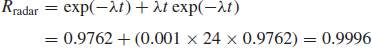
6.6 Systems Reliability Models

6.6.1 The Basic Series Reliability Model

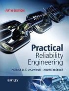
Consider a system composed of two independent components, each exhibiting a constant hazard (or failure) rate. If the failure of either component will result in failure of the system, the system can be represented by a reliability block diagram (RBD) (Figure 6.1). (A reliability block diagram does not necessarily represent the system's operational logic or functional partitioning.)

If λ₁ and λ₂ are the hazard rates of the two components, the system hazard rate will be λ₁ + λ₂. Because the hazard rates are constant, the component reliabilities R₁ and R₂, over a time of operation t, are exp (−λ₁t) and exp (−λ₂t). The reliability of the system is the combined probability of no failure of either component, that is R₁R₂ = exp [−(λ₁ + λ₂)t]. In general, for a series of n independent components:

Figure 6.1 Series System.

where R_i is the reliability of the ith component. This is known as the product rule or series rule (see Eqn. 2.2):

This is the simplest basic model on which parts count reliability prediction is based.

The failure logic model of the overall system will be more complex if there are redundant subsystems or components. Also, if system failure can be caused by events other than component failures, such as interface problems, the model should specifically include these, for example as extra blocks.

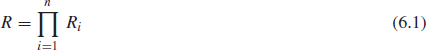
6.6.2 Active Redundancy

The reliability block diagram for the simplest redundant system is shown in Figure 6.2. In this system, composed of two independent parts with reliabilities R₁ and R₂, satisfactory operation occurs if either one or both parts function. Therefore, the reliability of the system, R, is equal to the probability of part 1 or part 2 surviving.

From Eqn. (2.6), the probability

This is often written

For the constant hazard rate case,

Figure 6.2 Dual redundant system.

The general expression for active parallel redundancy is

where R_i is the reliability of the ith unit and n the number of units in parallel. If in the two-unit active redundant system λ₁ = λ₂ = 0.1 failures per 1000 h, the system reliability over 1000 h is 0.9909. This is a significant increase over the reliability of a simple non-redundant unit, which is 0.9048. Such a large reliability gain often justifies the extra expense of designing redundancy into systems. The gain usually exceeds the range of prediction uncertainty. The example quoted is for a non-maintained system, that is the system is not repaired when one equipment fails. In practice, most active redundant systems include an indication of failure of one equipment, which can then be repaired. A maintained active redundant system is, of course, theoretically more reliable than a non-maintained one. Examples of non-maintained active redundancy can be found in spacecraft systems (e.g. dual thrust motors for orbital station-keeping) and maintained active redundancy is a feature of systems such as power generating systems and railway signals.

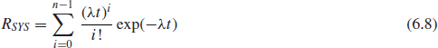
6.6.3 m-out-of-n Redundancy

In some active parallel redundant configurations, m out of the n units may be required to be working for the system to function. This is called m-out-of-n (or m/n) parallel redundancy. The reliability of an m/n system, with n independent components in which all the unit reliabilities are equal, is the binomial reliability function (based on Eq. 2.37):

or, for the constant hazard rate case:

6.6.4 Standby Redundancy

Standby redundancy sometimes referred as ‘cold standby’ is achieved when one unit does not operate continuously but is only switched on when the primary unit fails. A standby electrical generating system is an example. The block diagram in Figure 6.3 shows another. The standby unit and the sensing and switching system may be considered to have a ‘one-shot’ reliability R_s of starting and maintaining system function until the primary equipment is repaired, or R_s may be time-dependent. The switch and the redundant unit may have dormant hazard rates, particularly if they are not maintained or monitored.

Taking the case where the system is non-maintained, the units have equal constant operating hazard rates λ, there are no dormant failures and R_s = 1, then

Figure 6.3 Reliability block diagram for a missile system.

The general reliability formula for n equal units in a standby redundant configuration (perfect switching) is

If in a standby redundant system λ₁ = λ₂ = 0.1 failure per 1000 h, then the system reliability is 0.9953. This is higher than for the active redundant system [R(1000) = 0.9909], since the standby system is at risk for a shorter time. If we take into account less than perfect reliability for the sensing and switching system and possibly a dormant hazard rate for the standby equipment, then standby system reliability would be reduced.

6.6.5 Further Redundancy Considerations

The redundant systems described represent the tip of an iceberg as far as the variety and complexity of system reliability models are concerned. For systems where very high safety or reliability is required, more complex redundancy is frequently applied. Some examples of these are:

1. In aircraft, dual or triple active redundant hydraulic power systems are often used, with a further emergency (standby) back-up system in case of a failure of all the primary circuits.
2. Aircraft electronic flying controls typically utilize triple voting active redundancy. A sensing system automatically switches off one system if it transmits signals which do not match those transmitted by the other two, and there is a manual back-up system. The reliability evaluation must include the reliability of all three primary systems, the sensing system and the manual system.
3. Fire detection and suppression systems consist of detectors, which may be in parallel active redundant configuration, and a suppression system which is triggered by the detectors.

We must be careful to ensure that single-point failures which can partly eliminate the effect of redundancy are considered in assessing redundant systems. For example, if redundant electronic circuits are included within one integrated circuit package, a single failure such as a leaking hermetic seal could cause both circuits to fail. Such dependent failures are sometimes referred to as common mode (or common cause) failures, particularly in relation to systems. As far as is practicable, they must be identified and included in the analysis. Common mode failures are discussed in more detail later.

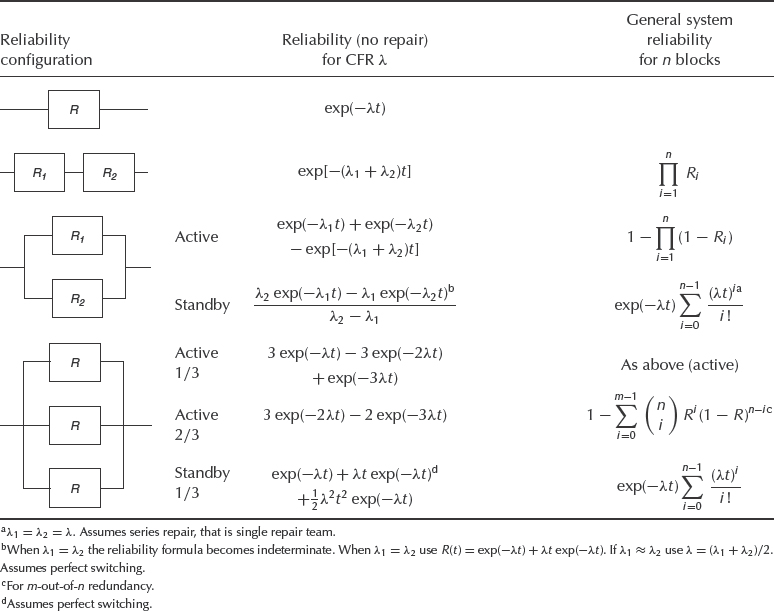
6.7 Availability of Repairable Systems

As mentioned in Section 2.15, there is a fundamental difference between the mathematical treatments of repairable and non-repairable systems. None of the commonly used statistical distributions can be applied to repairable systems due to the fact that failed units are not taken out of the population. This statement can be illustrated by a simple example where the number of repaired failures eventually exceeds the total number of parts in the field, thus making the cdf of a distribution greater than 1.0, which is mathematically impossible. Instead, repairable systems are modelled by a stochastic process. If a system can be repaired to ‘as good as new’ condition, then the appropriate model to describe the failure occurrence is called an ordinary renewal process (ORP) (see Section 2.15.2). If a system upon repair retains the same wearout characteristics as before it has a condition called ‘same as old’, and it is modelled by the non-homogeneous Poisson process (NHPP), see also Section 2.15.2. If the condition after repair is better than old, but worse than new (which is usually the case in real life), then it is modelled by the so-called generalized renewal process (GRP), see Kaminskiy and Krivtsov (2000) for more details.

Therefore, for a repairable system the ‘classic’ definition of reliability applies only to the time to first failure. Instead the reliability-equivalent of a repairable system is called availability. Availability is defined as the probability that an item will be available when required, or as the proportion of total time that the item is available for use. Therefore the availability of a repairable item is a function of its failure rate, λ, and of its repair or replacement rate μ. The difference between repairable and non-repairable systems is illustrated graphically in Figure 6.4.

The proportion of total time that the item is available (functional) is the steady-state availability. For a simple unit, with a constant failure rate λ and a constant mean repair rate μ, where μ = 1/MTTR (Mean Time to Repair), the steady-state availability is equal to:

The instantaneous availability or probability that the item will be available at time t is equal to

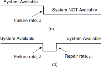
Figure 6.4 (a) Non-repairable system and (b) Repairable system.

Table 6.1 Reliability and availability for some systems configurations. (R. H. Myers, K. L. Wong and H. M. Gordy, Reliability Engineering for Electronic Systems, Copyright © 1964 John Wiley & Sons, Inc. Reprinted by permission of John Wiley & Sons, Inc.)

which approaches the steady-state availability as t becomes large. It is often more revealing, particularly when comparing design options, to consider system unavailability:

and

If scheduled maintenance is necessary and involves taking the system out of action, this must be included in the availability formula. The availability of spare units for repair by replacement is often a further consideration, dependent upon the previous spares usage and the repair rate of replacement units.

Availability is an important consideration in relatively complex systems, such as telecommunications and power networks, chemical plant and radar stations. In such systems, high reliability by itself is not sufficient to ensure that the system will be available when needed. It is also necessary to ensure that it can be repaired quickly and that essential scheduled maintenance tasks can be performed quickly, if possible without shutting down the system. Therefore maintainability is an important aspect of design for maximum availability, and trade-offs are often necessary between reliability and maintainability features. For example, built-in test equipment (BITE) is incorporated into many electronic systems. This added complexity can degrade reliability and can also result in spurious failure indications. However, BITE can greatly reduce maintenance times, by providing an instantaneous indication of fault location, and therefore availability can be increased. (This is not the only reason for the use of BITE. It can also reduce the need for external test equipment and for training requirements for trouble-shooting, etc.)

Availability is also affected by redundancy. If standby systems can be repaired or overhauled while the primary system provides the required service, overall availability can be greatly increased.

Table 6.1 shows the reliability and steady-state availability functions for some system configurations. It shows clearly the large gains in reliability and steady-state availability which can be provided by redundancy. However, these are relatively simple situations, particularly as a constant failure rate is assumed. Also, for the standby redundant case, it is assumed that:

1. The reliability of the changeover system is unity.
2. No common-cause failures occur.
3. Failures are detected and repaired as soon as they occur.

Of course, these conditions do not necessarily apply, particularly in the case of standby equipment, which must be tested at intervals to determine whether it is serviceable. The availability then depends upon the test interval. Monitoring systems are sometimes employed, for example, built-in test equipment (BITE) for electronic equipment, but this does not necessarily have a 100% chance of detecting all failures. In real-life situations it is necessary to consider these aspects, and the analysis can become very complex. Methods for dealing with more complex systems are given at the end of this chapter, and maintenance and maintainability are covered in more detail in Chapter 16.

Example 6.1

A shipboard missile system is composed of two warning radars, a control system, a launch and guidance system, and the missiles. The radars are arranged so that either can give warning if the other fails, in a standby redundant configuration. Four missiles are available for firing and the system is considered to be reliable if three out of four missiles can be fired and guided. Figure 6.3 shows the system in reliability block diagram form, with the MTBFs of the subsystems. The reliability of each missile is 0.9. Assuming that: (1) the launch and guidance system is constantly activated, (2) the missile flight time is negligible and (3) all elements are independent, evaluate: (a) the reliability of the system over 24 h, (b) the steady-state availability of the system, excluding the missiles, if the mean repair time for all units is 2 h and the changeover switch reliability is 0.95.

The reliabilities of the units over a 24 h period are:

1. The overall radar reliability is given by (from Table 6.1)

   

   The probability of the primary radar failing is (1 − R_P). The probability of this radar failing and the switch failing is the product of the two failure probabilities:

   

   Therefore the switch reliability effect can be considered equivalent to a series unit with reliability

   

   The system reliability, up to the point of missile launch, is therefore

   

   The reliability of any three out of four missiles is given by the cumulative binomial distribution (Eq. 6.5):

   

   The total system reliability is therefore

   

2. The availability of the redundant radar configuration is (see Table 6.1)

   

   The availability of the launch and guidance system

   

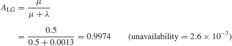
   The system availability is therefore

   

The previous example can be used to illustrate how such an analysis can be used for performing sensitivity studies to compare system design options. For example, a 20% reduction in the MTBF of the launch and guidance system would have a far greater impact on system reliability than would a similar reduction in the MTBF of the two radars.

In maintained systems which utilize redundancy for reliability or safety reasons, separate analyses should be performed to assess system reliability in terms of the required output and failure rate in terms of maintenance arisings. In the latter case all elements can be considered as being in series, since all failures, whether of primary or standby elements, lead to repair action.

Table 6.2 MTBR and replacement costs for the four modules.

Table 6.3 Cost per year of replacing the modules.

6.8 Modular Design

Availability and the cost of maintaining a system can also be influenced by the way in which the design is partitioned. ‘Modular’ design is used in many complex products, such as electronic systems and aero engines, to ensure that a failure can be corrected by a relatively easy replacement of the defective module, rather than by replacement of the complete unit.

Example 6.2

An aircraft gas turbine engine has a mean time between replacements (MTBR) – scheduled and unscheduled – of 1000 flight hours. With a total annual flying rate of 30 000 h and an average cost of replacement of $ 10 000, the annual repair bill amounted to $ 300 000. The manufacturer redesigned the engine so that it could be separated into four modules, with MTBR and replacement costs as shown in Table 6.2. What would be the new annual cost?

With the same total number of replacements, the annual repair cost is greatly reduced, from $ 300 000 to $ 72 750 (see Table 6.3).

Note that Example 6.2 does not take into account the different spares holding that would be required for the modular design (i.e. the operator would keep spare modules, instead of spare engines, thus making a further saving). In fact other factors would complicate such an analysis in practice. For example the different scheduled overhaul periods of the modules compared with the whole engine, the effect of wearout failure modes giving non-constant replacement rates with time since overhaul, and so on. Monte Carlo simulation is often used for planning and decision-making in this sort of situation (see Chapter 4).

6.9 Block Diagram Analysis

The failure logic of a system can be shown as a reliability block diagram (RBD), which shows the logical connections between components of the system. The RBD is not necessarily the same as a block schematic diagram of the system's functional layout. We have already shown examples of RBDs for simple series and parallel systems. For systems involving complex interactions construction of the RBD can be quite difficult, and a different RBD will be necessary for different definitions of what constitutes a system failure.

Figure 6.5 Block diagram decomposition.

Block diagram analysis consists of reducing the overall RBD to a simple system which can then be analysed using the formulae for series and parallel arrangements. It is necessary to assume independence of block reliabilities.

The technique is also called block diagram decomposition. It is illustrated in Example 6.3.

Example 6.3

The system shown in Figure 6.5 can be reduced as follows (assuming independent reliabilities):

6.9.1 Cut and Tie Sets

Complex RBDs can be analysed using cut set or tie set methods. A cut set is produced by drawing a line through blocks in the system to show the minimum number of failed blocks which would lead to system failure. Tie sets (or path sets) are produced by drawing lines through blocks which, if all were working, would allow the system to work. Figure 6.6 illustrates the way that cut and tie sets are produced. In this system there are three cut sets and two tie sets.

Approximate bounds on system reliability as derived from cut sets and tie sets, respectively, are given by

where N is the number of cut sets, T is the number of tie sets and n_j is the number of blocks in the jth cut set or tie set.

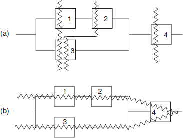
Figure 6.6 (a) Cut sets and (b) tie sets.

Example 6.4

Determine the reliability bounds of the system in Figure 6.6 for

Cut set:

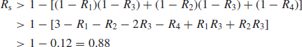
Tie set:

For comparison, the exact reliability is

The cut and tie set approaches are not used for systems as simple as in Example 6.4, since the decomposition approach is easy and gives an exact result. However, since the derivation of exact reliability using the decomposition approach can become an intractable problem for complex systems, the cut and tie set approach has its uses in such applications. The approximations converge to the exact system reliability as the system complexity increases, and the convergence is more rapid when the block reliabilities are high. Tie sets are not usually identified or evaluated in system analysis, however.

Cut and tie set methods are suitable for computer application. Their use is appropriate for the analysis of large systems in which various configurations are possible, such as aircraft controls, power generation, or control and instrumentation systems for large plant installations. The technique is subject to the constraint (as is the decomposition method) that all block reliabilities must be independent.

6.9.2 Common Mode Failures

A common mode (or common cause) failure is one which can lead to the failure of all paths in a redundant configuration. Identification and evaluation of common mode failures is very important, since they might have a higher probability of occurrence than the failure probability of the redundant system when only individual path failures are considered. In the design of redundant systems it is very important to identify and eliminate sources of common mode failures, or to reduce their probability of occurrence to levels an order or more below that of other failure modes.

For example, consider a system in which each path has a reliability R = 0.99 and a common mode failure which has a probability of non-occurrence R_CM = 0.98. The system can be designed either with a single unit or in a dual redundant configuration (Figure 6.7 (a) and (b)). Ignoring the common mode failure, the reliability of the dual redundant system would be 0.9999. However, the common mode failure practically eliminates the advantage of the redundant configuration.

Examples of sources of common mode failures are:

1. Changeover systems to activate standby redundant units.
2. Sensor systems to detect failure of a path.
3. Indicator systems to alert personnel to failure of a path.
4. Power or fuel supplies which are common to different paths.
5. Maintenance actions which are common to different paths, for example, an aircraft engine oil check after which a maintenance technician omits to replace the oil seal on all engines. (This has actually happened twice, very nearly causing a major disaster each time.)
6. Operating actions which are common to different paths, so that the same human error will lead to loss of both.

   

   Figure 6.7 Effect of common mode failure.

7. Software which is common to all paths, or software timing problems between parallel processors.
8. ‘Next weakest link’ failures. Failure of one item puts an increased load on the next item in series, or on a redundant unit, which fails as a result.

Common mode failures can be very difficult to foresee, and great care must be taken when analysing safety aspects of systems to ensure that possible sources are identified.

6.9.3 Enabling Events

An enabling event is one which, whilst not necessarily a failure or a direct cause of failure, will cause a higher level failure event when accompanied by a failure. Like common mode failures, enabling events can be important and difficult to anticipate, but they must be considered. Examples of enabling events are:

1. Warning systems disabled for maintenance, or because they create spurious warnings.
2. Controls incorrectly set.
3. Operating or maintenance personnel following procedures incorrectly, or not following procedures.
4. Standby elements being out of action due to maintenance.

6.9.4 Practical Aspects

It is essential that practical engineering considerations are applied to system reliability analyses. The reliability block diagram implies that the ‘blocks’ are either ‘failed’ or operating, and that the logic is correct. Examples of situations in which practical and logical errors can occur are:

1. Two diodes (or two check valves) connected in series. If either fails open circuit (stuck closed), there will be no current (fluid) flow, so they will be in series from a reliability point of view. On the other hand, if either fails short circuit (or stuck open), the other will provide the required system function (current/fluid will flow in one direction), so they will be in parallel from a reliability point of view.
2. Two thermally activated switches (thermostats) wired in parallel to provide over-temperature protection for a system by starting a cooling fan, with backup in case of failure of one of the switches. This configuration might be modelled as two switches in parallel. However, practical engineering considerations that could make this simple model misleading or invalid are:
   • If one fails to close, the other will perform the protection function. However, there is no way of knowing that one has failed (without additional circuits or checks).
   • If one fails permanently closed, the fan would run continuously.
   • Since the two switches will operate at slightly different temperatures, one will probably do all the switching, so the duty will not be shared equally. If the one that switches first fails open, the contacts on the other might have degraded due to inactivity, so that it fails to switch.
   • If they do both switch about the same number of times, they might both deteriorate (contact wear) at the same rate, so that when one fails the other might fail soon after.
3. Data on the in-flight failure probabilities of aircraft engines are used to determine whether new types of commercial aircraft meet safety criteria (e.g. ‘extended twin overwater operations’ (ETOPS)). Engines might fail so that they do not provide power, but also in ways that cause consequential damage and possible loss of the aircraft. If the analyses consider only loss of power, they would be biased against twin-engine aircraft.
4. Common mode failures are often difficult to predict, but can dominate the real reliability or safety of systems. Maintenance work or other human actions are prime contributors. For example
   • The Chernobyl nuclear reactor accident was caused by the operators conducting an unauthorized test.
5. Unexpected combinations of events can occur. For example:
   • The Concorde crash was caused by debris on the runway causing tyre failure, and fragments of the tyre then pierced the fuel tank.
   • The explosion of the Boeing 747 (TWA Flight 800) over the Atlantic in July 1996 was probably caused by damage to an electrical cable, resulting in a short circuit which allowed high voltage to enter the fuel quantity indication system in the centre fuel tank, which caused arcing which in turn caused a fuel vapour explosion.
6. System failures can be caused by events other than failure of components or sub-systems, such as electromagnetic interference (Chapter 9), operator error, and so on.

These examples illustrate the need for reliability and safety analyses to be performed by engineers with practical knowledge and experience of the system design, manufacture, operation and maintenance.

6.10 Fault Tree Analysis (FTA)

Fault tree analysis (FTA) is a reliability/safety design analysis technique which starts from consideration of system failure effects, referred to as ‘top events’. The analysis proceeds by determining how these can be caused by individual or combined lower level failures or events.

Standard symbols are used in constructing an FTA to describe events and logical connections. These are shown in Figure 6.8. Figure 6.9 shows a simple BDA for a type of aircraft internal combustion engine. There are two ignition systems in an active parallel redundant configuration. The FTA (Figure 6.10) shows that the top event failure to start can be caused by either fuel flow failure, injector failure or ignition failure (three-input OR gate). At a lower level total ignition failure is caused by failure of ignition systems 1 and 2 (two-input AND gate).

In addition to showing the logical connections between failure events in relation to defined top events, FTA can be used to quantify the top event probabilities, in the same way as in block diagram analysis. Failure probabilities derived from the reliability prediction values can be assigned to the failure events, and cut set and tie set methods can be applied to evaluate system failure probability.

Note that a different FTA will have to be constructed for each defined top event which can be caused by different failure modes or different logical connections between failure events. In the engine example, if the top event is ‘unsafe for flight’ then it would be necessary for both ignition systems to be available before take-off, and gate A1 would have to be changed to an OR gate.

The FTA shown is very simple; a representative FTA for a system such as this, showing all component failure modes, or for a large system, such as a flight control system or a chemical process plant, can be very complex and impracticable to draw out and evaluate manually. Computer programs are used for generating and evaluating FTAs. These perform cutset analysis and create the fault-tree graphics. The use of computer programs for FTA provides the same advantages of effectiveness, economy and ease of iterative analysis as described for FMECA. The practical aspects of system reliability modelling described earlier apply equally to FTA.

Since FTA considers multiple, as well as single failure events, the method is an important part of most safety analyses.

Figure 6.8 Standard symbols used in fault tree analysis.

6.11 State-Space Analysis (Markov Analysis)

A system or component can be in one of two states (e.g. failed, non-failed), and we can define the probabilities associated with these states on a discrete or continuous basis, the probability of being in one or other at a future time can be evaluated using state-space (or state-time) analysis. In reliability and availability analysis, failure probability and the probability of being returned to an available state, failure rate and repair rate, are the variables of interest.

Figure 6.9 Reliability block diagram of engine.

Figure 6.10 FTA for engine (incomplete).

The best-known state-space analysis technique is Markov analysis. The Markov method can be applied under the following major constraints:

1. The probabilities of changing from one state to another must remain constant, that is, the process must be homogenous. Thus the method can only be used when a constant hazard or failure rate assumption can be justified.
2. Future states of the system are independent of all past states except the immediately preceding one. This is an important constraint in the analysis of repairable systems, since it implies that repair returns the system to an ‘as new’ condition.

Nevertheless, the Markov analysis can be usefully applied to system reliability, safety and availability studies, particularly to maintained systems for which BDA is not directly applicable, provided that the constraints described above are not too severe. The method is used for analysing complex systems such as power generation and communications. Computer programs are available for Markov analysis.

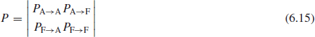
The Markov method can be illustrated by considering a single component, which can be in one of two states: failed (F) and available (A). The probability of transition from A to F is P_A→_F and from F to A is P_F →_A. Figure 6.11 shows the situation diagrammatically. This is called a state transition or a state-space diagram. All states, all transition probabilities and probabilities of remaining in the existing state ( = 1 − transition probability) are shown. This is a discrete Markov chain, since we can use it to describe the situation from increment to increment of time. Example 6.5 illustrates this.

Example 6.5

The component in Figure 6.11 has transitional probabilities in equal time intervals as follows:

What is the probability of being available after four time intervals, assuming that the system is initially available?

Figure 6.11 Two-state Markov state transition diagram.

Figure 6.12 Tree diagram for Example 6.5.

This problem can be solved by using a tree diagram (Figure 6.12).

The availability of the system is shown plotted by time interval in Figure 6.13. Note how availability approaches a steady state after a number of time intervals. This is a necessary conclusion of the underlying assumptions of constant failure and repair rates and of independence of events.

Whilst the transient states will be dependent upon the initial conditions (available or failed), the steady state condition is independent of the initial condition. However, the rate at which the steady state is approached is dependent upon the initial condition and on the transition probabilities.

6.11.1 Complex Systems

The tree diagram approach used above obviously becomes quickly intractable if the system is much more complex than the one-component system described, and analysed over just a few increments. For more complex systems, matrix methods can be used, particularly as these can be readily solved by computer programs. For example, for a single repairable component the probability of being available at the end of any time interval can be derived using the stochastic transitional probability matrix:

Figure 6.13 Transient availability of repaired system.

The stochastic transitional probability matrix for Example 6.5 is

The probability of being available after the first time increment is given by the first term in the first row (0.9), and the probability of being unavailable by the second term in the first row (0.1). To derive availability after the second time increment, we square the matrix:

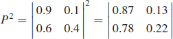
The probability of being available at the end of the second increment is given by the first term in the top row of the matrix (0.87). The unavailability = 1 – 0.87 = 0.13 (the second term in the top row).

For the third time increment, we evaluate the third power of the probability matrix, and so on.

Note that the bottom row of the probability matrix raised to the power 1, 2, 3, and so on, gives the probability of being available (first term) or failed (second term) if the system started from the failed state. The reader is invited to repeat the tree diagram (Figure 6.12), starting from the failed state, to corroborate this. Note also that the rows always summate to 1; that is, the total probability of all states. (Revision notes on simple matrix algebra are given in Appendix 7.)

If a system has more than two states (multi-component or redundant systems), then the stochastic transitional probability matrix will have more than 2 × 2 elements. For example, for a two-component system, the states could be:

The probabilities of moving from any one state to any other can be shown on a 4 × 4 matrix. If the transition probabilities are the same as for the previous example, then:

and the probability matrix is

The first two terms in the first row give the probability of being available and unavailable after the first time increment, given that the system was available at the start. The availability after 2, 3, and so on, intervals can be derived from p², p³, . . ., as above.

It is easy to see how, even for quite simple systems, the matrix algebra quickly diverges in complexity. However, computer programs can easily handle the evaluation of large matrices, so this type of analysis is feasible in the appropriate circumstances.

6.11.2 Continuous Markov Processes

So far we have considered discrete Markov processes. We can also use the Markov method to evaluate the availability of systems in which the failure rate and the repair rate (λ, μ) are assumed to be constant in a time continuum. The state transition diagram for a single repairable item is shown in Figure 6.14.

In the steady state, the stochastic transitional probability matrix is:

The instantaneous availability, before the steady state has been reached, can be derived using Eq. (6.11).

The methods described in the previous section can be applied for evaluating more complex, continuous Markov chains. The Markov analysis can also be used for availability analysis, taking account of the holdings and repair rate of spares. The reader should refer to Singh and Billinton (1977) and Pukite and Pukite (1998) for details of the Markov method as applied to more complex systems.

Figure 6.14 State–space diagram for a single-component repairable system.

6.11.3 Limitations, Advantages and Applications of Markov Analysis

The Markov analysis method suffers one major disadvantage. As mentioned earlier, it is necessary to assume constant probabilities or rates for all occurrences (failures and repairs). It is also necessary to assume that events are statistically independent. These assumptions are hardly ever valid in real life, as explained in Chapter 2 and earlier in this chapter. The extent to which they might affect the situation should be carefully considered when evaluating the results of a Markov analysis of a system.

The Markov analysis requires knowledge of matrix operations. This can result in difficulties in communicating the methods and the results to people other than reliability specialists. The severe simplifying assumptions can also affect the credibility of the results.

The Markov analysis is fast when run on computers and is therefore economical once the inputs have been prepared. The method is used for analysing systems such as power distribution networks and logistic systems.

6.12 Petri Nets

A further expansion of state-space analysis techniques came with development of Petri nets, which were introduced by Carl Adam Petri in 1962. A Petri net is a general-purpose graphical and mathematical tool for describing relations existing between conditions and events. The original Petri net did not include the concept of time, so that an enabled transition fires immediately (see Section 6.12.2). An extension called stochastic Petri nets (SPN) or time Petri nets was introduced in the late 1970s. Stochastic Petri nets address most of the shortcoming of Markov chains by focusing on modelling the states of components that comprise the system, so that the state of the system can be inferred from the states of its components rather than defined explicitly as required by the Markov approach.

SPN is often used as a modelling preprocessor, so the model is internally converted to Markov state space and solved using Markov methods. However, as mentioned before, the major disadvantage of the Markov method is its reliance on constant rates of all occurrences (Poisson process). In order to overcome that disadvantage and solve SPN directly, the Monte-Carlo method is often used to simulate the transition process. The original Petri nets are still used in software design, while reliability engineering uses mostly time Petri nets.

The basic symbols of Petri nets include:

: Place, drawn as a circle, denotes event.

: Immediate transition, drawn as a thin bar, denotes event transfer with no delay time.

: Timed transition, drawn as a thick bar, denotes event transfer with a period of delay time.

: Arc, drawn as an arrow, between places and transitions.

: Token, drawn as a dot, contained in places, denotes the data and also serves as an indicator of system's state.

: Inhibitor arc, drawn as a line with a circle end, between places and transitions.

The transition is said to fire if input places satisfy an enabled condition. Transition firing will remove one token from each of its input places and put one token into all of its output places. Basic structures of logic relations for Petri nets are listed in Figure 6.15, where there are two types of input places for the transition; namely, specified type and conditional type. The former one has single output arc whereas the latter has multiples. Tokens in the specified type place have only one outgoing destination, that is if the input place(s) holds a token then the transition fires and gives the output place(s) a token. However, tokens in the conditional type place have more than one outgoing paths that may lead the system to different situations. For the ‘TRANSFER OR’ Petri nets in Figure 6.15, whether Q or R takes over a token from P depends on conditions, such as probability, extra action, or self-condition of the place.

Figure 6.15 Basic structures of logic relations for Petri nets (Courtesy S. Yang).

There are three types of transitions that are classified based on time. Transitions with no time delay due to transition are called immediate transitions, while those needing a certain constant period of time for transition are called timed transitions. The third type is called a stochastic transition: it is used for modelling a process with random time. Owing to the variety of logical relations that can be represented with Petri nets, it is a powerful tool for modelling systems. Petri nets can be used not only for simulation, reliability analysis and failure monitoring, but also for dynamic behaviour observation. This greatly helps fault tracing and failure state analysis. Moreover, the use of Petri nets can improve the dialogue between analysts and designers of a system.

6.12.1 Transformation between Fault Trees and Petri Nets

Figure 6.16 is a fault tree example in which events A, B, C, D and E are basic causes of event 0. The logic relations between the events are described as well. The correlations between the fault tree and Petri net are shown in Figure 6.17.

Figure 6.18 is the Petri net transformation of Figure 6.16.

Figure 6.16 A fault tree (Courtesy S. Yang).

Figure 6.17 Correlations between fault tree and Petri net (Courtesy S. Yang).

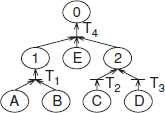
Figure 6.18 The Petri net transformation of Figure 6.16 (Courtesy S. Yang).

6.12.2 Minimum Cut Sets

To identify the minimum cut sets in a Petri net a matrix method is used, as follows:

1. Put down the numbers of the input places in a row if the output place is connected by multi-arcs from transitions. This accounts for OR-models.
2. If the output place is connected by one arc from a transition then the numbers of the input places should be put down in a column. This accounts for AND-models.
3. The common entry located in rows is the entry shared by each row.
4. Starting from the top event down to the basic events until all places are replaced by basic events, the matrix is thus formed, called the basic event matrix. The column vectors of the matrix constitute cut sets.
5. Remove the supersets from the basic event matrix and the remaining column vectors become minimum cut sets.

For example, the basic event matrix for Figure 6.18 is shown in Figure 6.19.

Figure 6.19 Minimum cut sets of Figure 6.18.

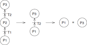
Figure 6.20 The absorption principle of equivalent Petri nets (Courtesy S. Yang).

Minimum cut sets can be derived in an opposite, bottom-up, direction, that is from basic places to the top place. Transitions with T = 0 are called immediate transitions. In a Petri net with immediate transitions, that is, the token transfers between places do not take time, then it can be absorbed to a simplified form called the equivalent Petri net.

Figure 6.20 shows the principle of absorption. After absorption, all the remaining places are basic events. The equivalent Petri net exactly constitutes the minimum cut sets, that is the input of each transition represents a minimum cut set.

6.12.3 Marking Transfer

A marking of a Petri net is defined as the total number of tokens at each place, denoted by a column vector M. Thus vector M_k = (n₁, n₂, . . ., n_m) represents that token numbers of places P₁, P₂, . . ., P_m at state k are n₁, n₂, . . ., n_m, respectively. Consequently, Petri nets can be expressed in state space form which gives the next state M_k+1 from its previous state M_k:

where M_k is the marking at state k, a m × 1 column vector, U_k is an input vector at state k, and A and B are matrix coefficients.

Since vector M_k represents the marking in a Petri net at state k, the failure state of a system may vary with time. Hence, the markings of a Petri net depend on time dynamically. The dynamic behaviour of system failure is defined as the system failure state with time varied, and is determined by the movement of tokens in the Petri net model. Thus, the dynamic behaviour of a system failure can be investigated by Petri nets whereas it cannot be done by fault trees. The method can be extended to include failure detection and correction logic, and repair and delay times. Since Petri net analysis is an emerging technical field, most of the software packages used for creating and analysing Petri nets are of a proprietary nature. Yakovlev et al. (2000) provides an introduction to Petri nets, and some applications have been described, for example in Yang and Liu (1997), Yang and Liu (1998) and Kleyner and Volovoi (2008).

Example 6.6

Let us consider an automotive airbag with a fault detection capability. When an airbag controller fails during regular driving conditions (no accident involved), a fault detection system detects that failure and turns the warning light on to inform the driver.

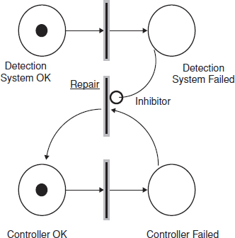
Figure 6.21 Petri net diagram for an airbag controller with a detection system (Kleyner and Volovoi, 2008).

Figure 6.21 depicts an airbag controller (bottom two places) and its detection system (top two places). When the controller fails, the bottom token moves to the right from the ‘Controller OK’ to ‘Controller Failed’ place. If the detection system functions properly, failure is detected by a driver, then repaired and the system is returned to the ‘Controller OK’ place via the ‘Repair’ transition in the middle. However if at some point the detection system fails, the top token moves from the ‘Detection System OK’ to ‘Detection System Failed’ place, which initiates an inhibitor disabling ‘Repair’ transition. Therefore if the controller fails now, the inhibitor will prevent the system from informing the driver about the failure and the controller will not be repaired. If the rates of each transition occurrence are constant, this system can be modelled as a Markov process. However if the rates are not constant (e.g. controller primary failures follow Weibull distribution) then the system should be modelled using Monte Carlo or other type of stochastic simulation.

6.13 Reliability Apportionment

Sometimes it is necessary to break an overall system reliability requirement down to individual subsystem reliabilities. This is common in large systems, particularly when different design teams or subcontractors are involved. The main contractor or system design team leader requires early assurance that subsystems will have reliabilities which will match the system requirement, and therefore the appropriate values have to be included in the subsystem specifications. This activity can be considered as a reliability ‘budgeting’.

The starting point for reliability apportionment is a reliability block diagram for the system drawn to show the appropriate system structure. The system requirement is then broken down in proportions which take account of the complexity, risk and existing experience related to each block. It is important to take account of the uncertainty inherent in such an early prediction, and therefore the block reliabilities need not aggregate to the system requirement, but to some higher reliability. The apportionment and specifications derived from it should take account of different operating conditions of subsystems. For example, a radar system might have a subsystem which operates for only half of the total system operating time, and therefore this should be shown on the RBD, and the failure rate apportioned to it should be related clearly either to the operating time of the system or of the subsystem.

6.14 Conclusions

System reliability (and safety and availability) prediction and modelling can be a frustrating exercise, since even quite simple systems can lead to complex reliability logic when redundancy, repair times, testing and monitoring are taken into account. On the other hand, the parameters used, particularly reliability values, are usually very uncertain, and can be highly variable between similar systems. This chapter has described some approaches, but it must be realized that the results can be very sensitive to parameter changes. For example, a single common-cause failure, overlooked in the analysis, might have a probability of occurrence which would completely invalidate the reliability calculations for a high reliability redundant system. In real life, availability is often determined more by spares holdings, administrative times (transport, documentation, delays, etc.) than by ‘predictable’ factors such as mean repair time. Therefore predictions and models of system reliability and availability should be used as a form of design review, to provide a disciplined framework for considering factors which will affect reliability and availability, and the sensitivity to changes in assumptions. Critical aspects can then be highlighted for further attention, and alternative system approaches can be compared.

Prediction and modelling are concepts which have generated much attention, literature and controversy in the reliability field. Considerable effort has been expended on the development and updating of databases and models, and a large proportion of the journal articles and conference contributions is devoted to the topics. Much of this work is of mainly academic interest, with limited practical applicability. The mathematical techniques described in this chapter are useful only in so far as the values inserted into the formulae are known within reasonably close limits. The use of complicated formulae to analyse the effects of parameters which are highly uncertain is inefficient and potentially misleading.

Finally, the predictions must be based on the commitment by the project management, and on a realistic appreciation of the technologies and risks.

Questions

1. Assume that you are responsible for the reliability aspects of a system containing both electronic and mechanical elements. The customer for the system requires that a numerical reliability prediction be provided:
   1. Describe what is meant by a ‘reliability prediction’ in this context.
   2. Identify some sources of data that can be used to assist in quantifying the prediction, and discuss the dangers that have to be guarded against in the use of such data.
   3. Do you expect the prediction to overestimate or underestimate the reliability that could be achieved by the system? Give your reasons.
2. Two resistors are connected in parallel in an electrical circuit. They can fail either open-circuit (resistance = ∞) or short-circuit (resistance = 0). Draw reliability block diagrams for the pair of resistors (i) for the circuit failing open-circuit; (ii) for the circuit failing-short circuit.
3. The system sketched below is used to regulate the downstream pressure of gas in a chemical plant. There are two regulators whose function is to keep the downstream pressure at a constant value. The upstream pressure fluctuates, but is always much higher than the required downstream pressure. The regulators function independently, but both sense the downstream pressure at the same point (X).

   

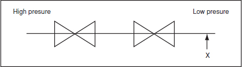
   A regulator can fail in one of two ways: ‘open’, in which case it becomes ‘straight through’ so that the flow of gas is unrestricted, and reliability in this mode is R₀; or ‘closed’, in which it totally blocks the flow of gas and reliability in this mode is R_c.

   1. On the assumption that the two types of failure are independent, produce expressions for system reliability (i) for the system failing due to total loss of flow; (ii) for the system failing due to overpressure downstream.
   2. The times to failure of the regulators are described by the following distributions: Closed – exponential with mean life 2 years.

      Open – Weibull with β = 1.8 and η = 1.6 years.

      What are the probabilities of the system giving one year of failure-free operation in each mode?

   3. What is the probability of obtaining one year of failure-free operation irrespective of the mode of failure?
4. It has been suggested that the reliability of the system in question 3 can be improved by adopting a twin-stream system as in the diagram below.

   

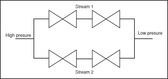
   Calculate the two system reliabilities for (loss of flow and overpressure) for this configuration.

5. Draw block diagrams for both modes of failure of the ‘twin stream’ in question 4. Draw the cut sets and tie sets in each case.
6. Calculate the reliability over a 150 h mission for the system whose reliability block diagram is shown below.

   

   The probability distributions of lives to failure of the elements are:

   1. constant hazard, mean life = 837 h.
   2. Weibull, with shape parameter = 2.0, characteristic life 315 h.
   3. normal, with mean = 420 h and standard deviation 133 h.
7. An element in a manufacturing system has a mean time between failures of 25 h. When it fails it takes, on average, 2 h to restore it to an operating condition. It has been suggested that the problems caused by the unreliability of this element could be avoided by installing a second identical element as a standby:
   1. Calculate the probability of completing an 8 h shift without a system failure both for the single-element and for the redundant-element system.
   2. If a repair team is made available such that repairs can be started on a failed element immediately after failure, calculate the long-term system availability (assuming continuous operation) for both the single-element and the redundant-element system. State all assumptions made and comment on whether you consider them reasonable.
   3. If the additional element costs £25 000 and downtime costs £100 per hour, what is the payback period for the additional element? (Ignore discounting of cash flows.)
8. In the context of fault-tree analysis, explain the meaning of each of the following:

   an AND gate	‘top’ event
   an OR gate	a basic event
   a priority AND gate	an undeveloped event.

   In each case, sketch the conventional symbol used and give a practical example.

9. A control system consists of an electrical power supply, a standby battery supply which is activated by a sensor and switch if the main supply fails, a hydraulic power pack, a controller, and two actuators acting in parallel (i.e. control exists if either or both actuators are functioning).
   1. Draw the system reliability block diagram.
   2. Draw the fault tree appropriate to the top event ‘total loss of actuator control’.
10. In question 9, if the reliabilities of the separate components are as follows:

    Main electrical supply: 0.99

    Standby battery supply: 0.995

    Sensor and switch: 0.995

    Hydraulic supply: 0.95

    Controller: 0.98

    Actuator (each): 0.99

    What is the system reliability for the top event ‘total loss of actuator control’?

11. This is a very simple example of simulation to explore the sort of principles involved in much more complex (and realistic) situations. It describes the common ‘queuing’ problem, but by using simulation we are able to circumvent the convenient, but often implausible assumptions that are usually incorporated in conventional ‘queuing theory’. In particular, we do not need to assume exponentially distributed arrival and service times.

    A radio taxi service operates between 9 a.m. and 7 p.m. Calls arrive at random at a rate of three per hour. The time to reach a customer is a Weibull distribution with β = 2, η = 0.25 h. The journey time is normally distributed with mean 30 minutes and standard deviation 6 minutes. A customer will only be offered a service if there is a taxi available, that is not currently on a journey.

    You are invited to do one ‘manual’ simulation of a day's operation with a fleet of two taxis, and evaluate the reliability (i.e. proportion of customers picked up). The calculations are simple but tedious, so computer methods are used when we want many thousands of simulations of much more complex situations. You will need to generate random sample values for:

    t₁ – the time of a customer call since the previous one.

    t₂ – the time to reach the customer.

    t₃ – the journey time with the customer.

    These will be developed from random numbers between 0 and 1. Such numbers can be generated in various ways; e.g:

    • doing Monte Carlo simulations (see Chapter 4).
    • using the ran# function on a calculator.
    • rolling a 20-sided die.
    • using tables of random numbers.
    • using the random number generator built into common application software (e.g. most spreadsheets). Simulating t₁:

    The reliability function (probability that the time to reach a customer exceeds t = t₁) is from the exponential distribution, that is = exp(−λt), from which t = 1/λ ln [1/R(t)]. Simply generate a random number between 0 and 1 for R(t) and calculate the value of t using λ = 1/3. For example, for a random number of 0.439, the random time is 3 ln (1/0.439) = 0.823 h.

    If running Monte Carlo simulation using Excel¯, use the functions in Chapter 4, Table 4.1 Simulating t₂:

    This time will be simulated from a Weibull distribution, where

    

    from which

    

    We have β = 2 and η = 0.25; so, for example, with a random number of 0.772, the simulated value of t₂ is

    

    If running Monte Carlo simulation using Excel¯, use the functions in Chapter 4, Table 4.1 Simulating t₃:

    This comes from a normal distribution. There is no closed form for the reliability function of this distribution, so some alternative approach is necessary. The easiest is to use tables of standardized random normal deviates (as included in most statistics books) or an implementation in a computer spreadsheet. Suppose we obtained a value of -0.194. For our particular normal distribution the mean is 0.5 h and the standard deviation 0.1 h, so the simulated random time is

    

    If running Monte Carlo simulation using Excel¯, use the functions in Chapter 4, Table 4.1

    Using these ideas, ‘walk through’ a random sample of one day of operation of two taxis. See how many requests were made, and how many were delivered to their destinations.

12. A device used in a ground radar system has age to failure that is described approximately by a Weibull distribution with mean life 83 h, shape parameter 1.5, and location parameter zero. When it fails it takes on average 3.5 h to repair:
    1. Calculate the reliability over a 25 h period, and the ‘steady state’ availability of the device.
    2. Calculate the reliability over 25 h, and the ‘steady state’ availability of a subsystem that consists of two of these devices in active parallel redundancy.
    3. Identify all assumptions made in these calculations, and discuss their validity.
    4. Explain the meaning of the ‘steady state availability’ in (a) and (b) above, and consider whether it gives the most suitable measure of availability in this example.
13. Describe the practical limitations of using methods such as BDA, FTA, Markov chains, and so on for assessing the reliability, in qualitative and in quantitative terms, of the following (Hint: in each case, first define the failure you are considering):
    1. A parachute (consider the canopy, the lines and the deployment mechanism).
    2. A microprocessor (consider the power input, the data input and output connections, and every transistor and capacitor).
    3. An electric motor.
    4. A mechanical assembly that consists of static parts bolted together.
    5. A train.
14. Calculate the failure rate for a generic ceramic capacitor 0.2 μF (circuit resistance 0.5 /Ω/V) operating at the ambient temperature T = 60°C in the ground mobile environment. The capacitor has two pins, hermetic package and is rated to operate at the maximum temperature of 100°C. Compare the results obtained using MIL-HDBK-217 with and other method such as Telcordia or IEC 62380.
15. Draw a Markov state-space diagram and a Petri net for a standby system covered in Section 6.6.4. Consider both perfect and imperfect switching.
16. At the early design stage you need to evaluate the future reliability of the product. Which reliability prediction method would you choose if you have:
    1. A bill of materials for an electronic system.
    2. Mechanical drawings of the system.
    3. Bill of materials and the knowledge of the stress factors for the electronic components, such as temperature, vibration, voltage, and so on.
    4. Electronic schematics.
    5. List of mechanical parts and the detailed drawings.
    6. Detailed information about device geometry, material properties and the applied stresses.
    7. Field return and warranty data for the previous model of the system with clear description of the differences between the models.
    8. Field return and warranty data for the previous model of the system with clear description of the differences in the environmental stresses between the two models.
17. Develop a Fault Tree Diagram a coffee maker, a hand calculator, a digital camera, a water heater, a lawnmower, a microwave oven, an electronic thermostat, TV remote control, a vacuum cleaner or other every day product. Provide at least three levels of the FTA tree depth counting the top event.
18. The system XYZ can be divided into subsystems and be represented by the block diagram in Figure 6.22.

    

    Figure 6.22 System XYZ block diagram.

    The failures of each subsystem are distributed according to the following statistical distributions:

    A – Exponential λ = 12.0 failures per million hours.

    B – Weibull, β = 2.0, η = 20 000 hours.

    C – Normal, μ = 1600 hours, σ = 100 hours.

    D – Lognormal, μ = 24, σ = 12.

    E – Weibull, β = 0.8, η = 10 000 hours.

    Calculate the system reliability at 1200 hours.

    Calculate the system reliability at 1600 hours.

    For the Blocks A, B and E determine which portion of the bathtub curve best describes each sub-system? Explain why.

19. If a system consists of four major serial subsystems and the required reliability is 0.9, what is the allocated reliability of each subsystem, assuming equal apportionment?
20. Compare the reliability of three parts at 10 years mark:

    Part A (R_A): Failures are exponentially distributed with failure rate of 0.58 failures per million hours.

    Consider 24 hrs per day operation.

    Part B (R_B): B₁₀ life equals 10 years.

    Part C (R_C): Failures are distributed according to Weibull distribution with β = 2.0 and η = 20.0 years.

21. Two identical and independent components form an active redundant (parallel) system. Each component's time to failure follows Weibull distribution with the parameters β and η. Derive the analytical expression for this system's hazard rate h(t).
22. Develop a fault tree and analyse a car's turn signal system whose failure could be caused by a battery failure (P_B = 0.11), broken connector (P_C = 0.05) or burnt out light bulb (P_L = 0.21). What is the probability of failure for the whole system?
23. A system with standby redundancy and perfect switching has a failure rate of 0.006 failures per hour for each subsystem: primary and standby. What is the reliability of the whole system at 60 hours?

Bibliography

Alion System Reliability Center (2011) PRISM. Available at: http://src.alionscience.com/prism/ (Accessed 22 March 2011)

Andrews, J. and Moss, T. (2002) Reliability and Risk Assessment, ASME Press.

British Standard, BS 5760 (1991) Reliability of Systems, Equipments and Components, British Standards Institution, London.

British Telecom (1995) HRD5, Handbook of Reliability Data for Electronic Components used in Telecommunication Systems.

CALCE (2011) Center for Advanced Life Cycle Engineering. Available at http://www.calce.umd.edu/ (Accessed 22 March 2011).

Dylis, D (2001) PRISM: A new approach to reliability prediction. Amer. Soc. Quality (ASQ) Reliability Review, 21(1), March issue.

Dylis, D. and Priore, M. (2001) A Comprehensive Reliability Assessment Tool for Electronic Systems, IIT Research/ Reliability Analysis Center, Rome NY, Available at: http://www.theriac.org/productsandservices/products/217plus/rams01.pdf

FIDES (2009) FIDES Guide 2009 Issue A. Available at http://fides-reliability.org/ (Accessed 22 March 2011)

Foucher, B., Boullié, J.B., Meslet, B. and Das, D. (2002) A review of reliability prediction methods for electronic devices. Microelectronics Reliability, 42(8), 1155–1162.

Høyland, A., Rausand, M. (2004) System Reliability Theory, Models and Statistical Methods, 2nd edn, Wiley.

IEEE Standard 1413.1-2002 (2003) IEEE Guide for Selecting and Using Reliability Predictions Based on IEEE 1413, IEEE.

Kaminskiy, M. and Krivtsov, V. (2000) G-Renewal Process as a Model for Statistical Warranty Claim Prediction. Proceedings of the Annual Reliability and Maintainability Symposium (RAMS).

Kleyner, A. and Volovoi, V. (2008) Reliability Prediction using Petri Nets for On-Demand Safety Systems with Fault Detection, in Safety and Reliability and Risk Analysis (eds Martorell, Soares and Barnett), (European Safety and Reliability conference), v.3, pp. 1961–1968.

Kleyner, A. and Bender, M. (2003) Reliability Prediction Method Based on Merging Military Standards Approach with Manufacturer's Warranty Data. Proceedings of Annual Reliability and Maintainability Symposium (RAMS), Tampa, Florida, pp. 202–206.

Kleyner, A. and Boyle, J. (2003) Reliability Prediction of Substitute Parts Based on Component Temperature Rating and Limited Accelerated Test Data. Proceedings of Annual Reliability and Maintainability Symposium, Tampa, Florida, pp. 518–522.

McLeish, J. (2010) Enhancing MIL-HDBK-217 Reliability Predictions with Physics of Failure Methods. Proceedings of the Annual Reliability and Maintainability Symposium (RAMS).

MIL-HDBK-217F (1995) Military Handbook, Reliability Prediction of Electronic Equipment, Notice 2, Department of Defense, Washington, DC.

Nicholls, D. (2007) What is 217Plus™ and Where Did it Come From? Proceedings of the Annual Reliability and Maintainability Symposium (RAMS).

Nippon Telegraph and Telephone Corporation (1985) Standard Reliability Table for Semiconductor Devices.

NSWC-06/LE10 (2006) Handbook of Reliability Prediction Procedures for Mechanical Equipment, Edition 2006. US Naval Surface Warfare Center, Carderock Division, West Bethesda, Maryland 20817-5700. Available at: http://www.everyspec.com/USN/NSWC/NSWC-06_RELIAB_HDBK_2006_15051/.

Pukite J. and Pukite P. (1998) Markov Modelling for Reliability Analysis, IEEE Press.

RAIC (2010) Electronic Reliability Prediction. Available at http://www.theriac.org/DeskReference/viewDocument.php?id=211 (Accessed 22 March 2011).

RAIC (2011) 217Plus: RAIC's Reliability Prediction Methodology. Available at http://www.theriac.org/productsandservices/products/217plus/ (Accessed 22 March 2011).

ReliaSoft (2006) Standards Based Reliability Prediction in a Nutshell. Reliability Hotwire Issue 70, http://www.weibull.com/hotwire/issue70/relbasics70.htm (Accessed 22 March 2011).

Singh, C. and Billinton, R. (1977) System Reliability Modeling and Evaluation, Hutchinson.

Talmor, M. and Arueti, S. (1997) Reliability Prediction: The Turn-Over Point. Proceedings of Reliability and Maintainability Symposium (RAMS).

Telcordia Special Report SR-332 (2001) Reliability Prediction Procedure for Electronic Equipment (RPP). Issue 1, Telcordia Customer Service, Piscataway, NJ.

UTEC80810 (2000) Modele universel pour le calcul de la fiabileite previsionnelle des composants, cartes et equipememts electroniques – RDF2000.

Yakovlev, A., Gomes, L. and Lavagno, L. (2007) Hardware Design and Petri Nets, Kluwer Academic Publishers.

Yang, S. and Liu, T. (1997) Failure Analysis for an Airbag Inflator by Petri Nets. Quality and Reliability Engineering International, 13, 139–151.

Yang, S. and Liu, T. (1998) A Petri Net Approach to Early Failure Detection and Isolation for Preventive Maintenance. Quality and Reliability Engineering International, 14, 319–330.