16

Maintainability, Maintenance and Availability

16.1 Introduction

Most engineered systems are maintained, that is they are repaired when they fail, and work is performed on them to keep them operating. The ease with which repairs and other maintenance work can be carried out determines a system's maintainability.

Maintained systems may be subject to corrective and preventive maintenance (CM and PM). Corrective maintenance includes all action to return a system from a failed to an operating or available state. The amount of corrective maintenance is therefore determined by reliability. Corrective maintenance action usually cannot be planned; we must repair failures when they occur, though sometimes repairs can be deferred.

Corrective maintenance can be quantified as the mean time to repair (MTTR). The time to repair, however, includes several activities, usually divided into three groups:

1. Preparation time: finding the person for the job, travel, obtaining tools and test equipment, and so on.
2. Active maintenance time: actually doing the job.
3. Delay time (logistics time): waiting for spares, and so on, once the job has been started.

Active maintenance time includes time for studying repair charts, and so on, before the actual repair is started, and time spent in verifying that the repair is satisfactory. It might also include time for post-repair documentation when this must be completed before the equipment can be made available, for example on aircraft. Corrective maintenance is also specified as a mean active repair time (MART) or mean active corrective maintenance time (MACMT), since it is only the active time (excluding documentation) that the designer can influence.

Preventive maintenance seeks to retain the system in an operational or available state by preventing failures from occurring. This can be by servicing, such as cleaning and lubrication, or by inspection to find and rectify incipient failures, for example by crack detection or calibration. Preventive maintenance affects reliability directly. It is planned and should be performed when we want it to be. Preventive maintenance is measured by the time taken to perform the specified maintenance tasks and their specified frequency.

Maintainability affects availability directly. The time taken to repair failures and to carry out routine preventive maintenance removes the system from the available state. There is thus a close relationship between reliability and maintainability, one affecting the other and both affecting availability and costs.

The maintainability of a system is clearly governed by the design. The design determines features such as accessibility, ease of test, diagnosis and repair and requirements for calibration, lubrication and other preventive maintenance actions.

This chapter describes how maintainability can be optimized by design, and how it can be predicted and measured. It also shows how plans for preventive maintenance can be optimized in relation to reliability, to minimize downtime and costs.

16.2 Availability Measures

In order to analyse a system's availability it needs to be measured. Depending on the available data and the objectives of the analysis availability can be expressed in several different ways.

16.2.1 Inherent Availability

Inherent availability is the steady state availability which considers only the corrective maintenance (CM) (covered in Section 6.7). Assuming that CM actions occur at a constant rate, it can be estimated as:

MTBF is the mean time between failure and MTTR is the mean time to repair (Chapter 6) which is the same as mean corrective maintenance time.

16.2.2 Achieved Availability

Achieved availability is very similar to inherent availability with the exception that PM downtimes are also included. Specifically, it is the steady state availability in an ideal support environment (i.e. readily available tools, spares, personnel, etc.) The achieved availability is sometimes referred to as the availability seen by the maintenance department (does not include logistic delays, supply delays or administrative delays).

Achieved availability can be computed by looking at the mean time between maintenance actions MTBMA (both preventive and corrective) and the mean maintenance time, MMT:

Assuming constant failure rate MTBMA can be calculated as:

where: λ = the failure rate (assuming all failures are repaired).

The mean maintenance time MMT can be further decomposed into the effects of preventive and corrective maintenance as:

Where MTTR is the mean CM time and MPMT is the mean PM time.

16.2.3 Operational Availability

Operational availability is a measure of the ‘real’ average availability over a period of time in an actual operational environment. It includes all experienced sources of downtime, such as administrative downtime, logistic downtime, and so on

where: MDT = Mean maintenance downtime.

For more on availability measures see Blanchard and Fabrycky (2011).

Example 16.1

Calculate the achieved availability for a system with the demonstrated failure rate of 1 failure per 1000 hours of operation. Preventive maintenance is scheduled every 500 hours of operation and on average takes 6 hours. To repair a failed system takes on average 16 hours.

The frequency of preventive maintenance is f_PM = 1/500 h = 0.002 h⁻¹ and the failure rate is λ = 1/1000 h = 0.001 h⁻¹. Next step is to calculate MTBMA, MMT, and A_A based on (16.2)–(16.4).

16.3 Maintenance Time Distributions

Maintenance times tend to be lognormally distributed (see Figure 16.1). This has been shown by analysis of data. It also fits our experience and intuition that, for a task or group of tasks, there are occasions when the work is performed rather quickly, but it is relatively unlikely that the work will be done in much less time than usual, whereas it is relatively more likely that problems will occur which will cause the work to take much longer than usual. This skews time-to-repair distributions to the right.

In addition to the job-to-job variability, leading typically to a lognormal distribution of repair times, there is also variability due to learning. Depending upon how data are collected, this variability might be included in the job-to-job variability, for example if technicians of different experience are being used simultaneously. However, both the mean time and the variance should reduce with experience and training.

The properties of the lognormal distribution are described in Chapter 2.

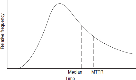
Figure 16.1 The lognormal distribution of maintenance times.

16.4 Preventive Maintenance Strategy

The effectiveness and economy of preventive maintenance can be maximized by taking account of the time-to-failure distributions of the maintained parts and of the failure rate trend of the system.

In general, if a part has a decreasing hazard rate, any replacement will increase the probability of failure. If the hazard rate is constant, replacement will make no difference to the failure probability. If a part has an increasing hazard rate, then scheduled replacement at any time will in theory improve reliability of the system. However, if the part has a failure-free life (Weibull γ < 0), then replacement before this time will ensure that failures do not occur. These situations are shown in Figure 16.2.

These are theoretical considerations. They assume that the replacement action does not introduce any other defects and that the time-to-failure distributions are exactly defined. As explained in Chapters 2 and 6, these assumptions must not be made without question. However, it is obviously of prime importance to take account of the time-to-failure distributions of parts in planning a preventive maintenance strategy.

In addition to the effect of replacement on reliability as theoretically determined by considering the time-to-failure distributions of the replaced parts, we must also take account of the effects of the maintenance action on reliability. For example, data might show that a high pressure hydraulic hose has an increasing hazard rate after a failure-free life, in terms of hose leaks. A sensible maintenance policy might therefore be to replace the hose after, say, 80% of the failure-free life. However, if the replacement action increases the probability of hydraulic leaks from the hose end connectors, it might be more economical to replace hoses on failure.

The effects of failures, both in terms of effects on the system and of costs of downtime and repair, must also be considered. In the hydraulic hose example, for instance, a hose leak might be serious if severe loss of fluid results, but end connector leaks might generally be only slight, not affecting performance or safety. A good example of replacement strategy being optimized from the cost point of view is the replacement of incandescent and fluorescent light units. It is cheaper to replace all units at a scheduled time before an expected proportion will have failed, rather than to replace each unit on failure, in large installations such as offices and street lights. However, at home we would replace only on failure.

Figure 16.2 Theoretical reliability and scheduled replacement relationships.

In order to optimize preventive replacement, it is therefore necessary to know the following for each part:

1. The time-to-failure distribution parameters for the main failure modes.
2. The effects of all failure modes.
3. The cost of failure.
4. The cost of scheduled replacement.
5. The likely effect of maintenance on reliability.

   

   Figure 16.3 RCM logic.

   We have considered so far parts which do not give any warning of the onset of failure. If incipient failure can be detected, for example by inspection, non-destructive testing, and so on, we must also consider:

6. The rate at which defects propagate to cause failure.
7. The cost of inspection or test.

Note that, from 2, an FMECA is therefore an essential input to maintenance planning.

This systematic approach to maintenance planning, taking account of reliability aspects, is called reliability centred maintenance (RCM). Figure 16.3 shows the basic logic of the method. RCM is widely applied, for example on aircraft, factory systems, and so on. It is described in Moubray (1999), Bloom (2005) and other books. RCM software is also available.

Example 16.2

A flexible cable on a robot assembly line has a time-to-failure distribution which is Weibull, with β = 1.7, η = 300 h and γ = 150 h. If failure occurs whilst in use the cost of stopping the line and replacing the cable is $ 5000. The cost of replacement during scheduled maintenance is $; 500. If the line runs for 5000 hours a year and scheduled maintenance takes place every week (100 hours), what would be the annual expected cost of replacement at one-weekly or two-weekly intervals?

With no scheduled replacement the probability of a failure occurring in t hours will be

With scheduled replacement after m hours, the scheduled maintenance cost in 5000 h will be

and the expected failure cost in each scheduled replacement interval will be (assuming not more than one failure in any replacement interval):

Then the total cost per year

Results are as follows:

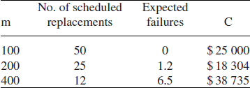
Therefore the optimum policy might be to replace the cables at alternate scheduled maintenance intervals, taking a slight risk of failure. (Note that the example assumes that not more than one failure occurs in any scheduled maintenance interval. If m is only a little more than γ this is a reasonable assumption.)

A more complete analysis could be performed using Monte Carlo simulation (Chapter 4). We could then take account of more detailed maintenance policies; e.g. it might be decided that if a cable had been replaced due to failure shortly before a scheduled maintenance period, it would not be replaced at that time.

16.4.1 Practical Implications

The time-to-failure patterns of components in a system therefore largely dictate the optimum maintenance policy. Generally, since most electronic components do not wear out, scheduled tests and replacements do not improve reliability. Indeed they are more likely to induce failures (real or reported). Electronic equipment should only be subjected to periodic test or calibration when drifts in parameters or other failures can cause the equipment to operate outside specification without the user being aware. Built-in test and auto-calibration can reduce or eliminate the need for periodic test.

Mechanical equipment subject to wear, corrosion, fatigue, and so on, should be considered for preventive maintenance.

16.5 FMECA and FTA in Maintenance Planning

The FMECA is an important prerequisite to effective maintenance planning and maintainability analysis. As shown earlier, the effects of failure modes (costs, safety implications, detectability) must be considered in determining scheduled maintenance requirements. The FMECA is also a very useful input for preparation of diagnostic procedures and checklists, since the likely causes of failure symptoms can be traced back using the FMECA results. When a fault tree analysis (FTA) has been performed it can also be used for this purpose.

16.6 Maintenance Schedules

When any scheduled maintenance activity is determined to be necessary, we must also determine the most suitable intervals between its performance. Maintenance schedules should be based upon the most appropriate time or other base. These can include:

• Road and rail vehicles: distance travelled.
• Aircraft: hours flown, numbers of takeoff/landing cycles.
• Electronic equipment: hours run, numbers of on/off cycles.
• Fixed systems (factory equipment, communications networks, rail infrastructure, etc.): calendar time.

The most appropriate base is the one that best accounts for the equipment's utilization in terms of the causes of degradation (wear, fatigue, parameter change, etc.), and is measured. For example, we measure the distance travelled by our cars, and most degradation is related to this. On the other hand, there is no point in setting a calibration schedule based upon running time for a measuring instrument unless an automatic or manual record of its utilization were maintained, so these are usually calendar-based.

16.7 Technology Aspects

16.7.1 Mechanical

Monitoring methods are used to provide periodic or continuous indications of the condition of mechanical components and systems. These include:

• Non-destructive test (NDT) for detection of fatigue cracks.
• Temperature and vibration monitors on bearings, gears, engines, and so on.
• Oil analysis, to detect signs of wear or breakup in lubrication and hydraulic systems.

16.7.2 Electronic and Electrical

Most electronic components and assemblies generally do not degrade in service, so long as they are protected from environments such as corrosion. Most electronic components and connections do not suffer from wear or fatigue, except as discussed in Chapter 9, so there is very seldom a pronounced ‘wearout’ phase in which failures become more likely or frequent. Therefore, apart from calibration for items like measuring instruments, scheduled tests are seldom appropriate.

16.7.3 ‘No Fault Found’

A large proportion of the reported failures of many electronic systems are not confirmed on later test. These occurrences are called no fault found (NFF) or re-test OK (RTOK) faults. Other terms used include No Trouble Found (NTF) and Customer Complaint Not Verified (CCNV). There are several causes of these, including:

• Intermittent failures, such as components that fail under certain conditions (temperature, etc.), intermittent opens on conductor tracks or solder connections, and so on.
• Tolerance effects, which can cause a unit to operate correctly in one system or environment but not in another.
• Connector troubles. The failure seems to be cleared by replacing a unit, when in fact it was caused by the connector, that is disturbed to replace it.
• Built-in test (BIT) systems which falsely indicate failures that have not actually occurred (see below).
• Failures that have not been correctly diagnosed and repaired, so that the symptoms recur.
• Inconsistent test criteria between the in-service test and the test applied during diagnosis elsewhere such as the repair depot.
• Human error or inexperience.
• In some systems, the diagnosis of which item (card, box) has failed might be ambiguous, so more than one is replaced even though only one has failed. Sometimes it is quicker and easier for the technician to replace multiple items, rather than trying to find out which has failed. In these cases multiple units are sent for diagnosis and repair, resulting in a proportion being classified NFF. (Returning multiple units can sometimes be justified economically. e.g., it might be appropriate to spend the minimum time diagnosing the cause of a problem on a system such as an aircraft or oil rig, in order to return the system to operation as soon as possible.).

The proportion of reported failures that are caused in these ways can be very high, often over 50% and sometimes up to 80%. This can generate high costs, in relation to warranty, spares, support, test facilities, and so on. NFF rates can be minimized by effective management of the design in relation to in-service test, and of the diagnosis and repair operations. Stress screening of repaired items can also reduce the proportion of failures that are not correctly diagnosed and repaired.

16.7.4 Software

As discussed in Chapter 10 software does not fail in the ways that hardware can, so there is no ‘maintenance’. If it is found to be necessary to change a program for any reason (change in system requirements, correction of a software error), this is really redesign of the program, not repair. So long as the change is made to all copies in use, they will all work identically, and will continue to do so.

16.7.5 Built-in Test (BIT)

Complex electronic systems such as laboratory instruments, avionics, communications networks and process control systems now frequently include built-in test (BIT) facilities. BIT consists of additional hardware and software which is used for carrying out functional test on the system. BIT might be designed to be activated by the operator, or it might monitor the system continuously or at set intervals.

BIT can be very effective in increasing system availability and user confidence in the system. However, BIT inevitably adds complexity and cost and can therefore increase the probability of failure. Additional sensors might be needed as well as BIT circuitry and displays. In microprocessor-controlled systems BIT can be largely implemented in software.

BIT can also adversely affect apparent reliability by falsely indicating that the system is in a failed condition. This can be caused by failures within the BIT, such as failures of sensors, connections, or other components. BIT should therefore be kept simple, and limited to monitoring of essential functions which cannot otherwise be easily monitored.

It is important to optimize the design of BIT in relation to reliability, availability and cost. Sometimes BIT performance is specified (e.g. ‘90% of failures must be detected and correctly diagnosed by BIT’). An FMECA can be useful in checking designs against BIT requirements since BIT detection can be assessed against all the important failure modes identified.

16.8 Calibration

Calibration is the regular check or test of equipment used for measuring physical parameters, by making comparisons against standard sources. Calibration is applied to basic measurement tools such as micrometers, gauges, weights and torque wrenches, and to transducers and instruments that measure parameters such as flow rate, electrical potential, current and resistance, frequency, and so on. Therefore calibration may involve simple comparisons (weight, timekeeping, etc.) or more complex testing (radio frequency, engine torque, etc.).

Whether an item needs to be calibrated or not depends primarily upon its application, and also upon whether or not inaccuracy would be apparent during normal use. Any instrument used in manufacturing should be calibrated, to ensure that correct measurements are being made. Calibration is often a legal requirement, for example of measuring systems in food or pharmaceutical production and packaging, retailing, safety–critical processes, and so on.

Calibration requirements and systems are described in Morris (1997).

16.9 Maintainability Prediction

Maintainability prediction is the estimation of the maintenance workload which will be imposed by scheduled and unscheduled maintenance. A standard method used for this work is US MIL-HDBK-472 which contains four methods for predicting the mean time to repair (MTTR) of a system. Method II is the most frequently used. This is based simply on summing the products of the expected repair times of the individual failure modes, t_r and dividing by the sum of the individual failure rates, that is:

The same approach is used for predicting the mean preventive maintenance time, with λ replaced by the frequency of occurrence of the preventive maintenance action.

MIL-HDBK-472 describes the methods to be used for predicting individual task times, based upon design considerations such as accessibility, skill levels required, and so on. It also describes the procedures for calculating and documenting the analysis, and for selection of maintenance tasks when a sampling basis is to be used (method III), rather than by considering all maintenance activities, which is impracticable on complex systems.

16.10 Maintainability Demonstration

A standard approach to maintainability demonstration is MIL-HDBK-470. The technique is the same as for maintainability prediction using method III of MIL-HDBK-472, except that the individual task times are measured rather than estimated from the design. Selection of task times to be demonstrated might be by agreement or by random selection from a list of maintenance activities. For more on maintainability demonstration see Blanchard and Fabrycky (2011).

16.11 Design for Maintainability

It is obviously important that maintained systems are designed so that maintenance tasks are easily performed, and that the skill levels required for diagnosis, repair and scheduled maintenance are not too high, considering the experience and training of likely maintenance personnel and users. Features such as ease of access and handling, the use of standard tools and equipment rather than specials, and the elimination of the need for delicate adjustment or calibration are desirable in maintained systems. As far as is practicable, the need for scheduled maintenance should be eliminated. Whilst the designer has no control over the performance of maintenance people, he or she can directly affect the inherent maintainability of a system.

Design rules and checklists should include guidance, based on experience of the relevant systems, to aid design for maintainability and to guide design review teams.

Design for maintainability is closely related to design for ease of production. If a product is easy to assemble and test maintenance will usually be easier. Design for testability of electronic circuits is particularly important in this respect, since circuit testability can greatly affect the ease and accuracy of failure diagnosis, and thus maintenance and logistics costs. Design of electronic equipment for testability is covered in more detail in Chapter 9.

Interchangeability is another important aspect of design for ease of maintenance of repairable systems. Replaceable components and assemblies must be designed so that no adjustment or recalibration is necessary after replacement. Interface tolerances must be specified to ensure that replacement units are interchangeable.

16.12 Integrated Logistic Support

Integrated logistic support (ILS) is a concept developed by the military, in which all aspects of design and of support and maintenance planning are brought together, to ensure that the design and the support system are optimized. Operational effectiveness, availability, and total costs of deployment and support are all considered. The approach is described in US-MIL-HDBK 1388, and in Jones (2006).

ILS, and the associated logistic support analysis (LSA), require inputs of reliability and maintainability data and forecasts, as well as data on costs, weights, special tools and test equipment, training requirements, and so on. MIL-HDBK-1388 requires that all analyses are computerized, and lays down standard input and output formats. Several commercial computer programs have been developed for the tasks.

ILS/LSA outputs are obviously very sensitive to the accuracy of the inputs. In particular, reliability forecasts can be highly uncertain, as explained in Chapter 6. Therefore such analyses, and decisions based upon them, should take full account of these uncertainties.

Questions

1. Define and explain the following terms: (a) availability; (b) maintainability; (c) condition monitoring.
2. 1. a Explain circumstances in which it is possible to improve maintainability to counteract poor reliability, and also identify circumstances where this approach is unrewarding.
   2. The expression for steady-state availability of a single element is:

      

      Explain what is meant by a steady state. State the meanings of the symbols μ and λ, and the assumptions inherent in the expression.

3. Describe the concept of reliability centred maintenance (RCM), including the key inputs to the analysis.
4. Recommend a planned replacement policy for the pumps in question 4 in Chapter 3.
5. Detail the time-related activities you may consider when analysing a maintenance-related task. (Hint: break the time down into active (or uptime) and inactive (or downtime)).
6. The median (50th percentile) active time to restore/repair a system after failure, using specified procedures and resources, is not to be more than 4.5 h. The maximum 15% active restore/repair time should not be more than 13.5 h (i.e. mean repair time = 5.7 h). Criticize the statement given and deduce what would be a realistic set of consistent numbers. You should use the following equations related to the log-normal distribution: ]

   

   Where t_MART is the mean time to repair, t_m the median time to repair, and t_α the ‘maximum’ time to repair, evaluated at the (1 − α) percentile point on the distribution. Z_α is the standardized normal deviate found in Appendix 1, and σ is the standard deviation of the distribution.

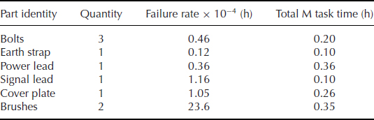
7. Given the removal and replacement time data in the table, calculate t_MART (mean time to repair)

   

8. Calculate the operational availability for a power generator with 1 scheduled maintenance per 1000 hours of operation and failure rate of 0.6 failures per 1000 hours. Preventive maintenance takes on average 8 hours, however if the engine fails, it typically takes 26 hours to repair it. Logistics and administrative delays typically add extra 12 hours to the maintenance time.
9. Solve problem 8 with maintenance times distributed lognormally. For corrective maintenance times μ = 3.3 and σ = 0.6 and for preventive maintenance μ = 2.2 and σ = 0.4.
10. How will the routine replacement of parts, which have a constant hazard rate, affect their field failure rate? Justify your answer.
11. A wave soldering machine failures follow 3-parameter Weibull distribution with β = 1.6, η = 800 hours and γ = 500 hours. The cost of one PM is $ 6000 and the cost of an unexpected failure is $ 16 000. The machine operates 24 hours/day and PMs are done every three months. Determine the yearly cost for this maintenance schedule.

Bibliography

Blanchard, B. and Fabrycky, W. (2011) Systems Engineering and Analysis, 5th edn, Prentice Hall.

Bloom, N. (2005) Reliability Centered Maintenance (RCM): Implementation Made Simple, McGraw-Hill.

Dhillon, B. (1999) Engineering Maintainability; How to Design for Reliability and Easy Maintenance, Gulf Publishing.

Jardine, A. and Tsang, A. (2005) Maintenance, Replacement and Reliability. Dekker.

Jones, J. (2006) Integrated Logistics Support Handbook, McGraw-Hill Logistics Series.

Morris, A. (1997) Measurement and Calibration Requirements for Quality Assurance to ISO9000, Wiley.

Moubray, J. (1999) Reliability Centred Maintenance, 2nd edn, Butterworth-Heinemann.

Smith, D. (2005) Reliability, Maintainability, and Risk, 7th edn, Elsevier.

UK Defence Standard 00–40. The Management of Reliability and Maintainability. HMSO.

US MIL-HDBK-1388. Integrated Logistic Support. Available from the National Technical Information Service, Springfield, Virginia.

US MIL-HDBK-470. Maintainability Program Requirements. Available from the National Technical Information Service, Springfield, Virginia.

US MIL-HDBK-472. Maintainability Prediction. Available from the National Technical Information Service, Springfield, Virginia.