One of the key tasks in designing a neural network application is to select appropriate inputs. For the unsupervised case, one wishes to use only relevant variables on which the neural network will find the patterns. And for the supervised case, there is a need to map the outputs to the inputs, so one needs to choose only the input variables which somewhat have influence on the output.
One strategy that helps in selecting good inputs in the supervised case is the correlation between data series, which is implemented in Chapter 5, Forecasting Weather. A correlation between data series is a measure of how one data sequence reacts or influences the other. Suppose we have one dataset containing a number of data series, from which we choose one to be an output. Now we need to select the inputs from the remaining variables.
The correlation takes values from -1 to 1, where values near to +1 indicate a positive correlation, values near -1 indicate a negative correlation, and values near 0 indicate no correlation at all.
As an example, let's see three charts of two variables X and Y:

In the first chart, to the left, visually one can see that as one variable decreases, the other increases its value (corr. -0.8). The middle chart shows the case when the two variables vary in the same direction, therefore positive correlation (corr. +0.7). The third chart, to the right, shows a case where there is no correlation between the variables (corr. -0.1).
There is no threshold rule as to which correlation should be taken into account as a limit; it depends on the application. While absolute correlation values greater than 0.5 may be suitable for one application, in others, values near 0.2 may add a significant contribution.
Linear correlation is very good in detecting behaviors between data series when they are presumably linear. However, if two data series form a parable when plotted together, linear correlation won't be able to identify any relation. That's why sometimes we need to transform data into a view that exhibits a linear correlation.
Data transformation depends on the problem that is being faced. It consists of inserting an additional data series with processed data from one or more data series. One example is an equation (possibly nonlinear) that includes one or more parameters. Some behaviors are more detectable under a transformed view of the data.
Another interesting point is regarding removing redundant data. Sometimes this is desired when there is a lot of available data in both unsupervised and supervised learning. As an example, let's see a chart of two variables:

It can be seen that both X and Y variables share the same shape, so this can be interpreted as a redundancy, as both variables are carrying almost the same information due the high positive correlation. Thus, one can consider a technique called Principal Component Analysis (PCA) which gives a good approach for dealing with these cases.
The result of PCA will be a new variable summarizing the previous two (or more). Basically, the original data series are subtracted by the mean and then multiplied by the transposed eigenvectors of the covariance matrix:

Here, SXY is the covariance between the variables X and Y.
The derived new data will be then:
Let's see now what a new variable would look like in a chart, compared to the original ones:

In our framework, we are going to add the class PCA that will perform this transformation and preprocessing before applying the data into a neural network:
public class PCA {

  DataSet originalDS;
  int numberOfDimensions;
  DataSet reducedDS;

  DataNormalization normalization = new DataNormalization(DataNormalization.NormalizationTypes.ZSCORE);

  public PCA(DataSet ds,int dimensions){
    this.originalDS=ds;
    this.numberOfDimensions=dimensions;
  }

  public DataSet reduceDS(){
    //matrix algebra to calculate transformed data in lower dimension
    …
  }

  public DataSet reduceDS(int numberOfDimensions){
    this.numberOfDimensions = numberOfDimensions;
    return reduceDS;
  }

}Noisy data and bad data are also sources of problems in neural network applications; that's why we need to filter data. One of the common data filtering techniques can be performed by excluding the records that exceed the usual range. For example, temperature values are between -40 and 40, so a value such as 50 would be considered an outlier and could be taken out.
The 3-sigma rule is a good and effective measure for filtering. It consists in filtering the values that are beyond three times the standard deviation from the mean:

Let's add a class to deal with data filtering:
public abstract class DataFiltering {

  DataSet originalDS;
  DataSet filteredDS;

}

public class ThreeSigmaRule extends DataFiltering {

  double thresholdDistance = 3.0;

  public ThreeSigmaRule(DataSet ds,double threshold){
    this.originalDS=ds;
    this.thresholdDistance=threshold;
  }

  public DataSet filterDS(){
    //matrix algebra to calculate the distance of each point in each column
    …
  }

}
These classes can be called in DataSet by the following methods, which are then called elsewhere for filtering and reducing dimensionality:
public DataSet applyPCA(int dimensions){
  PCA pca = new PCA(this,dimensions);
  return pca.reduceDS();
}

public DataSet filter3Sigma(double threshold){
  ThreeSigmaRule df = new ThreeSigmaRule(this,threshold);
  return df.filterDS();
}Among a number of strategies for validating a neural network, one very important one is cross-validation. This strategy ensures that all data has been presented to the neural network as training and test data. The dataset is partitioned into K groups, of which one is separated for testing while the others are for training:

In our code, let's create a class called CrossValidation to manage cross-validation:
public class CrossValidation {
  NeuralDataSet dataSet;
  int numberOfFolds;

  public LearningAlgorithm la;

  double[] errorsMSE;

  public CrossValidation(LearningAlgorithm _la,NeuralDataSet _nds,int _folds){
    this.dataSet=_nds;
    this.la=_la;
    this.numberOfFolds=_folds;
    this.errorsMSE=new double[_folds];
  }

  public void performValidation() throws NeuralException{
    //shuffle the dataset
    NeuralDataSet shuffledDataSet = dataSet.shuffle();
    int subSize = shuffledDataSet.numberOfRecords/numberOfFolds;
    NeuralDataSet[] foldedDS = new NeuralDataSet[numberOfFolds];
    for(int i=0;i<numberOfFolds;i++){
            foldedDS[i]=shuffledDataSet.subDataSet(i*subSize,(i+1)*subSize-1);
    }
    //run the training
    for(int i=0;i<numberOfFolds;i++){
      NeuralDataSet test = foldedDS[i];
      NeuralDataSet training = foldedDS[i==0?1:0];
      for(int k=1;k<numberOfFolds;k++){
        if((i>0)&&(k!=i)){
          training.append(foldedDS[k]);
        }
        else if(k>1) training.append(foldedDS[k]);
      }
      la.setTrainingDataSet(training);
      la.setTestingDataSet(test);
      la.train();
      errorsMSE[i]=la.getMinOverallError();
    }
  }
}To choose an adequate structure for a neural network is also a very important step. However, this is often done empirically, since there is no rule on how many hidden units a neural network should have. The only measure of how many units are adequate is the neural network performance. One assumes that if the general error is low enough, then the structure is suitable. Nevertheless, there might be a smaller structure that could yield the same result.
In this context, there are basically two methodologies: constructive and pruning. The constructive consists in starting with only the input and output layers, then adding new neurons at a hidden layer, until a good result can be obtained. The destructive approach, also known as pruning, works on a bigger structure on which the neurons having few contributions to the output are taken out.
The constructive approach is depicted in the following figure:

Pruning is the way back: when given a high number of neurons, one wishes to prune those whose sensitivity is very low, that is, whose contribution to the error is minimal:

To implement pruning, we`ve added the following properties in the class NeuralNet:
public class NeuralNet{
//…
  public Boolean pruning;
  public double senstitityThreshold;
}
A method called removeNeuron in the class NeuralLayer, which actually sets all the connections of the neuron to zero, disables weight updating and fires only zero at the neuron`s output. This method is called if the property pruning of the NeuralNet object is set to true. The sensitivity calculation is according to the chain rule, as shown in Chapter 3, Perceptrons and Supervised Learning and implemented in the calcNewWeigth method:
@Override
public Double calcNewWeight(int layer,int input,int neuron){
  Double deltaWeight=calcDeltaWeight(layer,input,neuron);
  if(this.neuralNet.pruning){
    if(deltaWeight<this.neuralNet.sensitivityThreshold)
      neuralNet.getHiddenLayer(layer).remove(neuron);
  }
  return newWeights.get(layer).get(neuron).get(input)+deltaWeight;
}