In this chapter, we are going to explore in more detail supervised learning, which is very useful in finding relations between two datasets. Also, we introduce perceptrons, a very popular neural network architecture that implements supervised learning. This chapter also presents their extended generalized version, the so-called multi-layer perceptrons, as well as their features, learning algorithms, and parameters. Also, the reader will learn how to implement them in Java and how to use them in solving some basic problems. This chapter will cover the following topics:
- Supervised learning
- Regression tasks
- Classification tasks
- Perceptrons
- Linear separation
- Limitations: the XOR problem
- Multilayer perceptrons
- Generalized delta rule – backpropagation algorithm
- Levenberg–Marquardt algorithm
- Single hidden layer neural networks
- Extreme learning machines
In the previous chapter, we introduced the learning paradigms that apply to neural networks, where supervised learning implies that there is a goal or a defined target to reach. In practice, we present a set of input data X, and a set of desired output data YT, then we evaluate a cost function whose aim is to reduce the error between the neural output Y and the target output YT.
In supervised learning, there are two major categories of tasks involved, which are detailed as follows: classification and regression.
Neural networks also work with categorical data. Given a list of classes and a dataset, one wishes to classify them according to a historical dataset containing records and their respective class. The following table shows an example of this dataset, considering the subjects' average grades between 0 and 10:
|
Student Id |
Subjects |
Profession | |||||||
|---|---|---|---|---|---|---|---|---|---|
|
English |
Math |
Physics |
Chemistry |
Geography |
History |
Literature |
Biology | ||
|
89543 |
7.82 |
8.82 |
8.35 |
7.45 |
6.55 |
6.39 |
5.90 |
7.03 |
Electrical Engineer |
|
93201 |
8.33 |
6.75 |
8.01 |
6.98 |
7.95 |
7.76 |
6.98 |
6.84 |
Marketer |
|
95481 |
7.76 |
7.17 |
8.39 |
8.64 |
8.22 |
7.86 |
7.07 |
9.06 |
Doctor |
|
94105 |
8.25 |
7.54 |
7.34 |
7.65 |
8.65 |
8.10 |
8.40 |
7.44 |
Lawyer |
|
96305 |
8.05 |
6.75 |
6.54 |
7.20 |
7.96 |
7.54 |
8.01 |
7.86 |
School Principal |
|
92904 |
6.95 |
8.85 |
9.10 |
7.54 |
7.50 |
6.65 |
5.86 |
6.76 |
Programmer |
One example is the prediction of profession based on scholar grades. Let's consider a dataset of former students who are now working. We compile a data set containing each student's average grade on each subject and his/her current profession. Note that the output would be the name of professions, which neural networks are not able to give directly. Instead, we need to make one column (one output) for each known profession. If that student chose a certain profession, the column corresponding to that profession would have the value one, otherwise it would be zero:

Now we want to find a model - based on a neural network - to predict which profession a student will be likely to choose based on his/her grades. To that end, we structure a neural network containing the number of scholar subjects as the input and the number of known professions as the output, and an arbitrary number of hidden neurons in the hidden layer:

For classification problems, there is usually only one class for each data point. So in the output layer, the neurons are fired to produce either zero or one, it being better to use activation functions that are output bounded between these two values. However, we must consider the case in which more than one neuron fires, giving two classes for a record. There are a number of mechanisms to prevent this case, such as the softmax function or the winner-takes-all algorithm, for example. These mechanisms are going to be detailed in the practical application in Chapter 6, Classifying Disease Diagnosis.
After being trained, the neural network has learned what will be the most probable profession for a given student given his/her grades.
Regression consists in finding some function that maps a set of inputs to a set of outputs. The following table shows how a dataset containing k records of m independent inputs X are known to be bound to n dependent outputs:
|
Input independent data |
Output dependent data | ||||||
|---|---|---|---|---|---|---|---|
|
X1 |
X2 |
… |
XM |
T1 |
T2 |
… |
TN |
|
x1[0] |
x2[0] |
… |
xm[0] |
t1[0] |
t2[0] |
… |
tn[0] |
|
x1[1] |
x2[1] |
… |
xm[1] |
t1[1] |
t2[1] |
… |
tn[1] |
|
… |
… |
… |
… |
… |
… |
… |
… |
|
x1[k] |
x2[k] |
… |
xm[k] |
t1[k] |
t2[k] |
… |
tn[k] |
The preceding table can be compiled in matrix format:

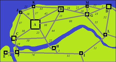
Unlike the classification, the output values are numerical instead of labels or classes. There is also a historical database containing records of some behavior we would like the neural network to learn. One example is the prediction of bus ticket prices between two cities. In this example, we collect information from a list of cities and the current ticket prices of buses departing from one and arriving to another. We structure the city features as well as the distance and/or time between them as the input and the bus ticket price as the output:
|
Features city of origin |
Features city of destination |
Features of the way between |
Ticket fare | ||||||
|---|---|---|---|---|---|---|---|---|---|
|
Population |
GDP |
Routes |
Population |
GDP |
Routes |
Distance |
Time |
Stops | |
|
500,000 |
4.5 |
6 |
45,000 |
1.5 |
5 |
90 |
1,5 |
0 |
15 |
|
120,000 |
2.6 |
4 |
500,000 |
4.5 |
6 |
30 |
0,8 |
0 |
10 |
|
30,000 |
0.8 |
3 |
65,000 |
3.0 |
3 |
103 |
1,6 |
1 |
20 |
|
35,000 |
1.4 |
3 |
45,000 |
1.5 |
5 |
7 |
0.4 |
0 |
5 |
|
… | |||||||||
|
120,000 |
2.6 |
4 |
12,000 |
0.3 |
3 |
37 |
0.6 |
0 |
7 |
Having structured the dataset, we define a neural network containing the exact number of features (multiplied by two, provided two cities) plus the route features in the input, one output, and an arbitrary number of neurons in the hidden layer. In the case presented in the preceding table, there would be nine inputs. Since the output is numerical, there is no need to convert output data.
This neural network would give an estimate price for a route between two cities, which currently is not served by any bus transportation company.