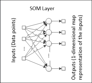
This network architecture was created by the Finnish professor Teuvo Kohonen at the beginning of the 80s. It consists of one single layer neural network capable of providing a visualization of the data in one or two dimensions.
In this book, we are going to use Kohonen networks also as a basic competitive layer with no links between the neurons. In this case, we are going to consider it as zero dimension (0-D).
Theoretically, a Kohonen Network would be able to provide a 3-D (or even in more dimensions) representation of the data; however, in printed material such as this book, it is not practicable to show 3-D charts without overlapping some data. Thus in this book, we are going to deal only with 0-D, 1-D, and 2-D Kohonen networks.
Kohonen Self-Organizing Maps (SOMs), in addition to the traditional single layer competitive neural networks (in this book, the 0-D Kohonen network), add the concept of neighborhood neurons. A dimensional SOM takes into account the index of the neurons in the competitive layer, letting the neighborhood of neurons play a relevant role during the learning phase.
An SOM has two modes of functioning: mapping and learning. In the mapping mode, the input data is classified in the most appropriate neuron, while in the learning mode, the input data helps the learning algorithm to build the map. This map can be interpreted as a lower-dimension representation from a certain dataset.
In our code, let's create a new class inherited from NeuralNet, since it will be a particular type of neural network. This class will be called Kohonen, which will use the class CompetitiveLayer as the output layer. The following class diagram shows how these new classes are arranged:

Three types of SOMs are covered in this chapter: zero-, one- and two-dimensional. These configurations are defined in an enum MapDimension:
public enum MapDimension {ZERO,ONE_DIMENSION,TWO_DIMENSION};The Kohonen constructor defines the dimension of the Kohonen neural network:
public Kohonen(int numberofinputs, int numberofoutputs, WeightInitialization _weightInitialization, int dim){
  weightInitialization=_weightInitialization;
  activeBias=false;
  numberOfHiddenLayers=0; //no hidden layers
//…
  numberOfInputs=numberofinputs;
  numberOfOutputs=numberofoutputs;
  input=new ArrayList<>(numberofinputs);
  inputLayer=new InputLayer(this,numberofinputs);
// the competitive layer will be defined according to the dimension passed in the argument dim
  outputLayer=new CompetitiveLayer(this,numberofoutputs, numberofinputs,dim);
  inputLayer.setNextLayer(outputLayer);
  setNeuralNetMode(NeuralNetMode.RUN);
  deactivateBias();
}This is the pure competitive layer, where the order of the neurons is irrelevant. Features such as neighborhood functions are not taken into account. Only the winner neuron weights are affected during the learning phase. The map will be composed only of unconnected dots.
The following code snippet define a zero-dimensional SOM:
int numberOfInputs=2;
int numberOfNeurons=10;
Kohonen kn0 = new Kohonen(numberOfInputs,numberOfNeurons,new UniformInitialization(-1.0,1.0),0);
Note the value 0 passed in the argument dim (the last of the constructor).
This architecture is similar to the network presented in the last section, Competitive learning, with the addition of neighborhood amongst the output neurons:
Note that every neuron on the output layer has one or two neighbors. Similarly, the neuron that fires the greatest value updates its weights, but in a SOM, the neighbor neurons also update their weights in a smaller rate.
The effect of the neighborhood extends the activation area to a wider area of the map, provided that all the output neurons must observe an organization, or a path in the one-dimensional case. The neighborhood function also allows for a better exploration of the properties of the input space, since it forces the neural network to keep the connections between neurons, therefore resulting in more information in addition to the clusters that are formed.
In a plot of the input data points with the neural weights, we can see the path formed by the neurons:

In the chart here presented, for simplicity, we plotted only the output weights to demonstrate how the map is designed in a (in this case) 2-D space. After training over many iterations, the neural network converges to a final shape that represent all data points. Provided that structure, a certain set of data may cause the Kohonen Network to design another shape in the space. This is a good example of dimensionality reduction, since a multidimensional dataset when presented to the Self-Organizing Map is able to produce one single line (in the 1-D SOM) that summarizes the entire dataset.
To define a one-dimensional SOM, we need to pass the value 1 as the argument dim:
Kohonen kn1 = new Kohonen(numberOfInputs,numberOfNeurons,new UniformInitialization(-1.0,1.0),1);
This is the most used architecture to demonstrate the Kohonen neural network power in a visual way. The output layer is one matrix containing M x N neurons, interconnected like a grid:

In the 2-D SOMs, every neuron now has up to four neighbors (in the square configuration), although in some representations, the diagonal neurons may also be considered, thus resulting in up to eight neighbors. Hexagonal representations are also useful. Let's see one example of what a 3x3 SOM plot looks like in a 2-D chart (considering two input variables):

At first, the untrained Kohonen Network shows a very strange and screwed-up shape. The shaping of the weights will depend solely on the input data that is going to be fed to the SOM. Let's see an example of how the map starts to organize itself:


The final shape of a 2-D SOM may not always be a perfect square; instead, it will resemble a shape that could be drawn from the dataset. The neighborhood function is one important component in the learning process because it approximates the neighbor neurons in the plot, and the structure moves to a configuration that is more organized.
In order to better represent the neurons of a 2D competitive layer in a grid form, we're creating the CompetitiveLayer2D class, which inherits from CompetitiveLayer. In this class, we can define the number of neurons in the form of a grid of M x N neurons:
public class CompetitiveLayer2D extends CompetitiveLayer {

    protected int sizeMapX; // neurons in dimension X
    protected int sizeMapY; // neurons in dimension Y

    protected int[] winner2DIndex;// position of the neuron in grid

    public CompetitiveLayer2D(NeuralNet _neuralNet,int numberOfNeuronsX,int numberOfNeuronsY,int numberOfInputs){
        super(_neuralNet,numberOfNeuronsX*numberOfNeuronsY,
numberOfInputs);
        this.dimension=Kohonen.MapDimension.TWO_DIMENSION;
        this.winnerIndex=new int[1];
        this.winner2DIndex=new int[2];
        this.coordNeuron=new int[numberOfNeuronsX*numberOfNeuronsY][2];
        this.sizeMapX=numberOfNeuronsX;
        this.sizeMapY=numberOfNeuronsY;
        //each neuron is assigned a coordinate in the grid
        for(int i=0;i<numberOfNeuronsY;i++){
            for(int j=0;j<numberOfNeuronsX;j++){
                coordNeuron[i*numberOfNeuronsX+j][0]=i;
                coordNeuron[i*numberOfNeuronsX+j][1]=j;
            }
        }
    }
The coordinate system in the 2D competitive layer is analogous to the Cartesian. Every neuron is assigned a position in the grid, with indexes starting from 0:

In the illustration above, 12 neurons are arranged in a 3 x 4 grid. Another feature added in this class is the indexing of neurons by the position in the grid. This allows us to get subsets of neurons (and weights), one entire specific row or column of the grid, for example:
public double[] getNeuronWeights(int x, int y){
  double[] nweights = neuron.get(x*sizeMapX+y).getWeights();
  double[] result = new double[nweights.length-1];
  for(int i=0;i<result.length;i++){
    result[i]=nweights[i];
  }
  return result;
}

public double[][] getNeuronWeightsColumnGrid(int y){
  double[][] result = new double[sizeMapY][numberOfInputs];
  for(int i=0;i<sizeMapY;i++){
    result[i]=getNeuronWeights(i,y);
  }
  return result;
}

public double[][] getNeuronWeightsRowGrid(int x){
  double[][] result = new double[sizeMapX][numberOfInputs];
  for(int i=0;i<sizeMapX;i++){
    result[i]=getNeuronWeights(x,i);
  }
  return result;
}A self-organizing map aims at classifying the input data by clustering those data points that trigger the same response on the output. Initially, the untrained network will produce random outputs, but as more examples are presented, the neural network identifies which neurons are activated more often and then their position in the SOM output space is changed. This algorithm is based on competitive learning, which means a winner neuron (also known as best matching unit, or BMU) will update its weights and its neighbor weights.
The following flowchart illustrates the learning process of a SOM Network:

The learning resembles a bit those algorithms addressed in Chapter 2, Getting Neural Networks to Learn and Chapter 3, Perceptrons and Supervised Learning. Three major differences are the determination of the BMU with the distance, the weight update rule, and the absence of an error measure. The distance implies that nearer points should produce similar outputs, thus here the criterion to determine the lowest BMU is the neuron which presents a lower distance to some data point. This Euclidean distance is usually used, and in this book we will apply it for simplicity:
The weight-to-input distance is calculated by the method getWeightDistance( ) of the CompetitiveLayer class for a specific neuron i (argument neuron). This method was described above.
The weight update rule uses a neighborhood function Θ(u,v,s,t) which states how much a neighbor neuron u (BMU unit) is close to a neuron v. Remember that in a dimensional SOM, the BMU neuron is updated together with its neighbor neurons. This update is also dependent on a neighborhood radius, which takes into account the number of epoch's s and a reference epoch t:

Here, du,v is the neuron distance between neurons u and v in the grid. The radius is calculated as follows:
Here, is the initial radius. The effect of the number of epochs (s) and the reference epoch (t) is the decreasing of the neighborhood radius and thereby the effect of neighborhood. This is useful because in the beginning of the training, the weights need to be updated more often, because they are usually randomly initialized. As the training process continues, the updates need to be weaker, otherwise the neural network will continue to change its weights forever and will never converge.
The neighborhood function and the neuron distance are implemented in the CompetitiveLayer class, with overridden versions for the CompetitiveLayer2D class:
|
CompetitiveLayer |
CompetitiveLayer2D |
|---|---|
public double neighborhood(int u, int v, int s,int t){
  double result;
  switch(dimension){
case ZERO:
  if(u==v) result=1.0;
  else result=0.0;
  break;
case ONE_DIMENSION:
default:
  double exponent=-(neuronDistance(u,v)
/neighborhoodRadius(s,t));
  result=Math.exp(exponent);
  }
  return result;
} |
@Override
public double neighborhood(int u, int v, int s,int t){
  double result;
  double exponent=-(neuronDistance(u,v)
/neighborhoodRadius(s,t));
  result=Math.exp(exponent);
  return result;
} |
public double neuronDistance(int u,int v){
  return Math.abs(coordNeuron[u][0]-coordNeuron[v][0]);
} |
@Override
public double neuronDistance(int u,int v){
  double distance=
Math.pow(coordNeuron[u][0]
-coordNeuron[v][0],2);
  distance+=
Math.pow(coordNeuron[u][1]-coordNeuron[v][1],2);
  return Math.sqrt(distance);
} |
The neighborhood radius function is the same for both classes:
public double neighborhoodRadius(int s,int t){
  return this.initialRadius*Math.exp(-((double)s/(double)t));
}
The learning rate also becomes weaker as the training goes on:
The parameter is the initial learning rate. Finally, considering the neighborhood function and the learning rate, the weight update rule is as follows:
Here, X k is the kth input, and W kj is the weight connecting the kth input to the jth output.
Now that we have a competitive layer, a Kohonen neural network, and defined the methods for neighboring functions, let's create a new class for competitive learning. This class will inherit from LearningAlgorithm and will receive Kohonen objects for learning:

As seen in Chapter 2, Getting Neural Networks to Learn a LearningAlgorithm object receives a neural dataset for training. This property is inherited by the CompetitiveLearning object, which implements new methods and properties to realize the competitive learning procedure:
public class CompetitiveLearning extends LearningAlgorithm {
    // indicates the index of the current record of the training dataset
    private int currentRecord=0;
    //stores the new weights until they will be applied
    private ArrayList<ArrayList<Double>> newWeights;
    //saves the current weights for update
    private ArrayList<ArrayList<Double>> currWeights;
    // initial learning rate
    private double initialLearningRate = 0.3;
    //default reference epoch
    private int referenceEpoch = 30;
    //saves the index of winner neurons for each training record
    private int[] indexWinnerNeuronTrain;
//…
}
The learning rate, as opposed to the previous algorithms, now changes over the training process, and it will be returned by the method getLearningRate( ):
public double getLearningRate(int epoch){
  double exponent=(double)(epoch)/(double)(referenceEpoch);
  return initialLearningRate*Math.exp(-exponent);
}
This method is used in the calcWeightUpdate( ):
@Override
public double calcNewWeight(int layer,int input,int neuron)
            throws NeuralException{
//…
  Double deltaWeight=getLearningRate(epoch);
  double xi=neuralNet.getInput(input);
  double wi=neuralNet.getOutputLayer().getWeight(input, neuron);
  int wn = indexWinnerNeuronTrain[currentRecord];
  CompetitiveLayer cl = ((CompetitiveLayer)(((Kohonen)(neuralNet))
                   .getOutputLayer()));
  switch(learningMode){
    case BATCH:
    case ONLINE: //The same rule for batch and online modes
      deltaWeight*=cl.neighborhood(wn, neuron, epoch, referenceEpoch) *(xi-wi);
      break;
  }
  return deltaWeight;
}
The train( ) method is adapted as well for competitive learning:
@Override
public void train() throws NeuralException{
//…
  epoch=0;
  int k=0;
  forward();
//…
  currentRecord=0;
  forward(currentRecord);
  while(!stopCriteria()){
    // first it calculates the new weights for each neuron and input
    for(int j=0;j<neuralNet.getNumberOfOutputs();j++){
      for(int i=0;i<neuralNet.getNumberOfInputs();i++){
        double newWeight=newWeights.get(j).get(i);
        newWeights.get(j).set(i,newWeight+calcNewWeight(0,i,j));
      }
    }
    //the weights are promptly updated in the online mode
    switch(learningMode){
      case BATCH:
        break;
      case ONLINE:
      default:
        applyNewWeights();
    }
    currentRecord=++k;
    if(k>=trainingDataSet.numberOfRecords){
      //for the batch mode, the new weights are applied once an epoch
      if(learningMode==LearningAlgorithm.LearningMode.BATCH){
        applyNewWeights();
      }
      k=0;
      currentRecord=0;
      epoch++;
      forward(k);
//…
    }
  }
}
The implementation for the method appliedNewWeights( ) is analogous to the one presented in the previous chapter, with the exception that there is no bias and there is only one output layer.
Time to play: SOM applications in action. Now it is time to get hands-on and implement the Kohonen neural network in Java. There are many applications of self-organizing maps, most of them being in the field of clustering, data abstraction, and dimensionality reduction. But the clustering applications are the most interesting because of the many possibilities one may apply them on. The real advantage of clustering is that there is no need to worry about input/output relationship, rather the problem solver may concentrate on the input data. One example of clustering application will be explored in Chapter 7, Clustering Customer Profiles.
In this section, we are going to introduce the plotting feature. Charts can be drawn in Java by using the freely available package JFreeChart (which can be downloaded from http://www.jfree.org/jfreechart/). This package is attached with this chapter's source code. So, we designed a class called Chart:
public class Chart {
  //title of the chart
  private String chartTitle;
  //datasets to be rendered in the chart
  private ArrayList<XYDataset> dataset = new ArrayList<XYDataset>();
  //the chart object
  private JFreeChart jfChart;
  //colors of each dataseries
  private ArrayList<Paint> seriesColor = new ArrayList<>();
  //types of series (dots or lines for now)
  public enum SeriesType {DOTS,LINES};
  //collections of types for each series
  public ArrayList<SeriesType> seriesTypes = new ArrayList<SeriesType>();

//…
}
The methods implemented in this class are for plotting line and scatter plots. The main difference between them lies in the fact that line plots take all data series over one x-axis (usually the time axis) where each data series is a line; scatter plots, on the other hand, show dots in a 2D plane indicating its position in relation to each of the axis. Charts below show graphically the difference between them and the codes to generate them:

int numberOfPoints=10;

double[][] dataSet = {
{1.0, 1.0},{2.0,2.0}, {3.0,4.0}, {4+.0, 8.0},{5.0,16.0}, {6.0,32.0},
{7.0,64.0},{8.0,128.0}};

String[] seriesNames = {"Line Plot"};
Paint[] seriesColor = {Color.BLACK};

Chart chart = new Chart("Line Plot", dataSet, seriesNames, 0, seriesColor, Chart.SeriesType.LINE);

ChartFrame frame = new ChartFrame("Line Plot", chart.linePlot("X Axis", "Y Axis"));

frame.pack();
frame.setVisibile(true);
int numberOfInputs=2;
int numberOfPoints=100;

double[][] rndDataSet =
RandomNumberGenerator
.GenerateMatrixBetween
(numberOfPoints
, numberOfInputs, -10.0, 10.0);
String[] seriesNames = {"Scatter Plot"};
Paint[] seriesColor = {Color.WHITE};

Chart chart = new Chart("Scatter Plot", rndDataSet, seriesNames, 0, seriesColor, Chart.SeriesType.DOTS);

ChartFrame frame = new ChartFrame("Scatter Plot", chart.scatterPlot("X Axis", "Y Axis"));

frame.pack();
We're suppressing the codes for chart generation (methods linePlot( ) and scatterPlot( )); however, in the file Chart.java, the reader can find their implementation.
Now that we have the methods for plotting charts, let's plot the training dataset and neuron weights. Any 2D dataset can be plotted in the same way shown in the diagram of the last section. To plot the weights, we need to get the weights of the Kohonen neural network using the following code:
CompetitiveLayer cl = ((CompetitiveLayer)(neuralNet.getOutputLayer()));
double[][] neuronsWeights = cl.getWeights();
In competitive learning, we can check visually how the weights move around the dataset space. So we're going to add a method (showPlot2DData( )) to plot the dataset and the weights, a property (plot2DData) to hold the reference to the ChartFrame, and a flag (show2DData) to determine whether the plot is going to be shown for every epoch:
protected ChartFrame plot2DData;

public boolean show2DData=false;

public void showPlot2DData(){
  double[][] data= ArrayOperations. arrayListToDoubleMatrix( trainingDataSet.inputData.data);
  String[] seriesNames = {"Training Data"};
  Paint[] seriesColor = {Color.WHITE};

  Chart chart = new Chart("Training epoch n°"+String.valueOf(epoch)+" ",data,seriesNames,0,seriesColor,Chart.SeriesType.DOTS);
  if(plot2DData ==null){
    plot2DData = new ChartFrame("Training",chart.scatterPlot("X","Y"));
  }

  Paint[] newColor={Color.BLUE};
  String[] neuronsNames={""};
  CompetitiveLayer cl = ((CompetitiveLayer)(neuralNet.getOutputLayer()));
  double[][] neuronsWeights = cl.getWeights();
  switch(cl.dimension){
    case TWO_DIMENSION:
      ArrayList<double[][]> gridWeights = ((CompetitiveLayer2D)(cl)). getGridWeights();
      for(int i=0;i<gridWeights.size();i++){
        chart.addSeries(gridWeights.get(i),neuronsNames, 0,newColor, Chart.SeriesType.LINES);
      }
      break;
    case ONE_DIMENSION:
      neuronsNames[0]="Neurons Weights";
      chart.addSeries(neuronsWeights, neuronsNames, 0, newColor, Chart.SeriesType.LINES);
      break;
    case ZERO:
      neuronsNames[0]="Neurons Weights";
    default:
      chart.addSeries(neuronsWeights, neuronsNames, 0,newColor, Chart.SeriesType.DOTS);
  }
  plot2DData.getChartPanel().setChart(chart.scatterPlot("X", "Y"));
}
This method will be called from the train method at the end of each epoch. A property called sleep will determine for how many milliseconds the chart will be displayed until the next epoch's chart replaces it:
if(show2DData){
  showPlot2DData();
  if(sleep!=-1)
    try{ Thread.sleep(sleep); }
    catch(Exception e){}
}Let's now define a Kohonen network and see how it works. First, we're creating a Kohonen with zero dimension:
RandomNumberGenerator.seed=0;
int numberOfInputs=2;
int numberOfNeurons=10;
int numberOfPoints=100;

// create a random dataset between -10.0 and 10.0
double[][] rndDataSet = RandomNumberGenerator. GenerateMatrixBetween(numberOfPoints, numberOfInputs, -10.0, 10.0);

// create the Kohonen with uniform initialization of weights
Kohonen kn0 = new Kohonen(numberOfInputs,numberOfNeurons,new UniformInitialization(-1.0,1.0),0);

//add the dataset to the neural dataset
NeuralDataSet neuralDataSet = new NeuralDataSet(rndDataSet,2);

//create an instance of competitive learning in the online mode
CompetitiveLearning complrn=new CompetitiveLearning(kn0,neuralDataSet, LearningAlgorithm.LearningMode.ONLINE);

//sets the flag to show the plot
complrn.show2DData=true;


try{
// give names and colors for the dataset
  String[] seriesNames = {"Training Data"};
  Paint[] seriesColor = {Color.WHITE};
  //this instance will create the plot with the random series
  Chart chart = new Chart("Training",rndDataSet,seriesNames,0, seriesColor);
  ChartFrame frame = new ChartFrame("Training", chart.scatterPlot("X", "Y"));
  frame.pack();
  frame.setVisible(true);

  // we pass the reference of the frame to the complrn object
  complrn.setPlot2DFrame(frame);
  // show the first epoch
  complrn.showPlot2DData();
//wait for the user to hit an enter
  System.in.read();
//training begins, and for each epoch a new plot will be shown
  complrn.train();
}
catch(Exception ne){

}
By running this code, we get the first plot:

As the training starts, the weights begin to distribute over the input data space, until finally it converges by being distributed uniformly along the input data space:

For one dimension, let's try something funkier. Let's create the dataset over a cosine function with random noise:
int numberOfPoints=1000;
int numberOfInputs=2;
int numberOfNeurons=20;
double[][] rndDataSet;

for (int i=0;i<numberOfPoints;i++){
  rndDataSet[i][0]=i;
  rndDataSet[i][0]+=RandomNumberGenerator.GenerateNext();
  rndDataSet[i][1]=Math.cos(i/100.0)*1000;
  rndDataSet[i][1]+=RandomNumberGenerator.GenerateNext()*400;
}
Kohonen kn1 = new Kohonen(numberOfInputs,numberOfNeurons,new UniformInitialization(0.0,1000.0),1);
By running the same previous code and changing the object to kn1, we get a line connecting all the weight points:

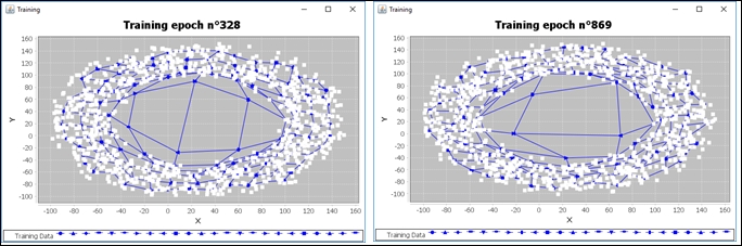
As the training continues, the lines tend to be organized along the data wave:

See the file Kohonen1DTest.java if you want to change the initial learning rate, maximum number of epochs, and other parameters.
Finally, let's see the two-dimensional Kohonen chart. The code will be a little bit different, since now, instead of giving the number of neurons, we're going to inform the Kohonen constructor the dimensions of our neural grid.
The dataset used here will be a circle with random noise added:
int numberOfPoints=1000;
for (int i=0;i<numberOfPoints;i++){
  rndDataSet[i][0]*=Math.sin(i);
  rndDataSet[i][0]+=RandomNumberGenerator.GenerateNext()*50;
  rndDataSet[i][1]*=Math.cos(i);
  rndDataSet[i][1]+=RandomNumberGenerator.GenerateNext()*50;
}
Now let's construct the two-dimensional Kohonen:
int numberOfInputs=2;
int neuronsGridX=12;
int neuronsGridY=12;
Kohonen kn2 = new Kohonen(numberOfInputs,neuronsGridX,neuronsGridY,new GaussianInitialization(500.0,20.0));
Note that we are using GaussianInitialization with mean 500.0 and standard deviation 20.0, that is, the weights will be generated at the position (500.0,500.0) while the data is centered around (50.0,50.0):

Now let's train the neural network. The neuron weights quickly move to the circle in the first epochs:

By the end of the training, the majority of the weights will be distributed over the circle, while in the center there will be an empty space, as the grid will be totally stretched out: