
Chapter 4
Iterative Source–Channel Decoding1
Code concatenation constitutes a convenient technique for constructing powerful codes capable of achieving huge coding gains, while keeping the decoding complexity manageable. The concept of Serially Concatenated Codes (SCCs) having an ‘outer’ and an ‘inner’ code used in cascade was proposed in [125]. The discovery of Parallel Concatenated ‘turbo’ Codes (PCCs) [69] considerably improved the achievable performance gains by separating component codes through interleavers and using iterative decoding in order to further reduce the BER. The intensive research efforts of the ensuing era demonstrated [70] that the employment of iterative processing techniques is not limited to traditional concatenated coding schemes. In other words, the ‘turbo principle’ [53] is applicable to numerous other algorithms that can be found in digital communications, for example in turbo equalization [82], spectrally efficient modulation [83, 84], turbo multiuser detection [87, 88] and channel-coded code-division multiple-access [90].
Previously, substantial research efforts have been focussed on optimizing concatenated coding schemes in order to improve the asymptotic slopes of their error probability curves, especially at moderate to high SNRs. Recently, researchers have focussed their efforts on investigating the convergence behavior of iterative decoding. In [77] the authors proposed a so-called density evolution algorithm for calculating the convergence thresholds of randomly constructed irregular LDPC codes designed for the AWGN channel. This method was used to study the convergence of iterative decoding for turbo-like codes in [104], where a SNR measure was proposed for characterizing the inputs and outputs of the component decoders. The mutual information between the data bits at the transmitter and the soft values at the receiver was used to describe the flow of extrinsic information between two soft-in soft-out decoders in [106]; the exchange of extrinsic information between constituent codes may be visualized as a staircase-shaped gradually increasing decoding trajectory within the EXIT charts of both parallel [98, 111] and serially concatenated codes [112]. A comprehensive study of the convergence behavior of iterative decoding schemes for bit-interleaved coded modulation, equalization and serially concatenated binary codes was presented in [115].
In this chapter we will investigate an intriguing application of the turbo principle [53], namely ISCD [42, 45, 252], where the channel decoder and the source decoder can be viewed as a pair of serial concatenated codes. By applying the turbo principle, the residual redundancy in the source after source encoding may be efficiently utilized for improving the system’s performance in comparison with that of separate source–channel decoding. Furthermore, the convergence behavior of various ISCD schemes will be analyzed with the aid of EXIT charts.
This chapter is organized as follows. Section 4.1 provides a brief introduction to various concatenated schemes and that of the iterative decoding principle: the turbo principle. The kernel of the turbo principle – the SISO APP decoding algorithm – and the semi-analytical tool of EXIT charts are described in Section 4.2. The achievable performance of the ISCD schemes is investigated in Sections 4.3 and 4.4, when communicating over AWGN channels and dispersive channels respectively. Section 4.5 concludes the chapter.
4.1 Concatenated Coding and the Turbo Principle
In this section we briefly describe several commonly used concatenated schemes, namely parallel concatenation [69,126] serial concatenation [71,130] and hybrid concatenation [253–255] of various constituent codes. Furthermore, we demonstrate that the turbo principle may be applied for detecting any of the above schemes.
4.1.1 Classification of Concatenated Schemes
4.1.1.1 Parallel Concatenated Schemes
The classic turbo codes [69] employ a parallel concatenated structure. Figure 4.1 shows two examples of the family of turbo codes. A so-called systematic code is shown in Figure 4.1a, where the input information bits are simply copied to the output, interspersed with the parity bits. By contrast a non-systematic code is shown in Figure 4.1b, where the original information bits do not explicitly appear at the output. The component encoders are often convolutional encoders, but binary Bose–Chaudhuri–Hocquenghem (BCH) codes [70] have also been used. At the encoder, the input information bits are encoded by the first constituent encoder (Encoder I) and an interleaved version of the input information bits is encoded by the second constituent encoder (Encoder II). The encoded output bits may be punctured, and hence arbitrary coding rates may be obtained. Furthermore, this structure can be extended to a parallel concatenation of more than two component codes, leading to multiple-stage turbo codes [126, 256].
4.1.1.2 Serially Concatenated Schemes
The basic structure of a SCC [71] is shown in Figure 4.2. The SCC encoder consists of an outer encoder (Encoder I) and an inner encoder (Encoder II), interconnected by an interleaver. The introduction of the interleaver scrambles the bits before they are passed to the other constituent encoder, which ensures that even if a specific bit has been gravely contaminated by the channel, the chances are that the other constituent decoder is capable of providing more reliable information concerning this bit. This is a practical manifestation of time diversity. Iterative processing is used in the SCC decoder, and a performance similar to that of a classic PCC may be achieved [71]. In fact, the serial concatenation constitutes quite a general structure and many decoding and detection schemes can be described as serially concatenated structures, such as those used in turbo equalization [82], coded modulation [83, 84], turbo multiuser detection [87, 88], joint source–channel decoding [42, 45, 252], LDPC decoding [77] and others[53,81]. Similarly, a serially concatenatedscheme may contain more than two components, as in [120–122, 130]. Figure 4.3 shows the schematic of a three-stage serially concatenated code [122, 130].
Figure 4.1: Two examples of parallel concatenated codes. The constituent codes are non-systematic codes having arbitrary code rates.
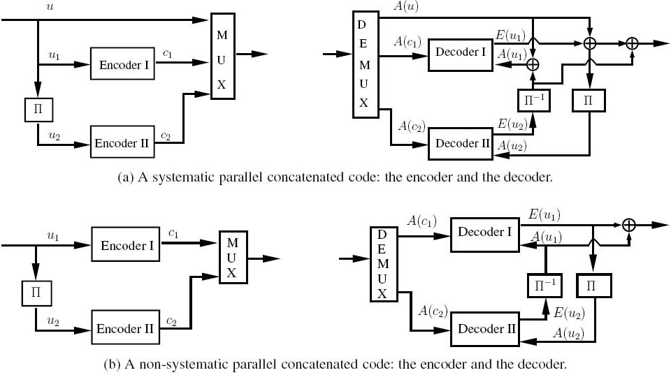
Figure 4.2: The schematic of a serially concatenated code: the encoder and the decoder.

Figure 4.3: The schematic of a three-stage serially concatenated code: the encoder and the decoder.

Figure 4.4: A trellis encoder, which processes the input information symbol sequence U and outputs encoded symbol sequence C. The encoder’s state transitions may be described by certain trellis diagrams.

4.1.1.3 Hybrid Concatenated Schemes
A natural extension of PCCs and SCCs is the family of hybrid concatenated codes [253–255], which combine the two principles. More specifically, some of the components are concatenated in parallel and some are serially concatenated. Again, the employment of this scheme is not restricted to channel coding. For example, combined turbo decoding and turbo equalization [257, 258] constitutes a popular application.
4.1.2 Iterative Decoder Activation Order
Since the invention of turbo codes [69], iterative (turbo) decoding has been successfully applied to diverse detection and decoding problems, which may inherit any of the three concatenated structures described above. Hence this technique has been referred to as the ‘Turbo Principle’ [53]. The crucial point at the receiver is that the component detectors or decoders have to be soft-in soft-out decoders that are capable of accepting and delivering probabilities or soft values, and the extrinsic part of the soft output of one of the decoders is passed on to the other decoder to be used as a priori input. If there are only two component decoders, the decoding alternates between them. When there are more component decoders, the activation order of the decoders is an important issue, which is sometimes referred to as ‘scheduling’ in the related literature – borrowing the terminology from the field of resource allocation. The specific activation order may substantially affect the decoding complexity, delay and performance of the system [121, 122].
4.2 SISOAPP Decoders and their EXIT Characteristics
The key point of iterative decoding of various concatenated schemes is that each component decoder employs a SISO algorithm. Benedetto et al.[254] proposed a SISO APP module, which implements the APP algorithm [48] in its basic form for any trellis-based decoder/detector. This SISO APP module is employed in our ISCD schemes in the rest of this treatise unless stated otherwise. Moreover, the capability of processing a priori information and generating extrinsic information is an inherent characteristic of a SISO APP module, which may be visualized by EXIT charts. Let us first introduce the SISO APP module.
4.2.1 A Soft-Input Soft-Output APP Module
4.2.1.1 The Encoder
Figure 4.4 shows a trellis encoder, which processes the input information symbol sequence U and outputs encoded symbol sequence C. The code trellis can be time invariant or time varying. For simplicity of exposition, we will refer to the case of binary time-invariant convolutional codes having code rate of R = k0/n0.
Figure 4.5: An edge of the trellis section.

The input symbol sequence U =(Uk)k∈![]() is defined over a symbol index set
is defined over a symbol index set ![]() and drawn from the alphabet U = {u1,...,uN I}. Each input symbol Uk consists of k0 bits Ukj, j = 1, 2,..., k0 with realization uj∈{0, 1}. The encoded output sequence C =(Ck)k∈
and drawn from the alphabet U = {u1,...,uN I}. Each input symbol Uk consists of k0 bits Ukj, j = 1, 2,..., k0 with realization uj∈{0, 1}. The encoded output sequence C =(Ck)k∈![]() of Figure 4.4 is defined over the same symbol index set
of Figure 4.4 is defined over the same symbol index set ![]() , and drawn from the alphabet C = {c1,...,cNo}. Each output symbol Ck consists of n0 bits Cjk, j = 1, 2,...,n0 with realization cj ∈ {0, 1}.
, and drawn from the alphabet C = {c1,...,cNo}. Each output symbol Ck consists of n0 bits Cjk, j = 1, 2,...,n0 with realization cj ∈ {0, 1}.
The legitimate state transitions of a time-invariant convolutional code are completely specified by a single trellis section, which describes the transitions (‘edges’) between the states of the trellis at time instants k and k + 1. A trellis section is characterized by:
- aset of N states
 = {s1,...,sN} (the state of the trellis at time k is Sk = s, with s∈S);
 - aset of N · NI edges obtained by the Cartesian product ε = × U = {e1,...,eN · NI}, which represent all legitimate transitions between the trellis states.
As seen in Figure 4.5, the following functions are associated with each edge e ∈ ε
- the starting state sS(e);
- the ending state sE(e);
- the input symbol u(e);
- the output symbol c(e).
The relationship between these functions depends on the particular encoder, while the assumption that the pair [sS(e),u(e)] uniquely identifies the ending state sE(e) should always be fulfilled, since it is equivalent to stating that, given the initial trellis state, there is a one-to-one correspondence between the input sequences and the state transitions.
4.2.1.2 The Decoder
The APP algorithm designed for the SISO decoder operates on the basis of the code’s trellis representation. It accepts as inputs the probabilities of each of the original information symbols and of the encoded symbols, labels the edges of the code trellis and generates as its outputs an updated version of these probabilities based upon the code constraints. Hence the SISO module may be viewed as a four-terminal processing block, as shown in Figure 4.6.
More specifically, we associate the sequence of information symbols u with the sequence of a priori probabilities P(u;I) = (Pk(u;I)) k∈![]() . Furthermore, we associate the sequence of encoded symbols c with the sequence of a priori probabilities p(c;I)=(Pk(c;I))k∈k, where we have
. Furthermore, we associate the sequence of encoded symbols c with the sequence of a priori probabilities p(c;I)=(Pk(c;I))k∈k, where we have ![]() The assumption that the a priori probabilities of specific symbols can be represented as the product of the probabilities of its constituent bits may be deemed valid when sufficiently long independent bit interleavers, rather than symbol interleavers, are used in the iterative decoding scheme of a concatenated code. The two outputs of the SISO module are the updated probabilities P(u; O) and P(c; O). Here, the letters I and O refer to the input and the output of the SISO module of Figure 4.6 respectively.
The assumption that the a priori probabilities of specific symbols can be represented as the product of the probabilities of its constituent bits may be deemed valid when sufficiently long independent bit interleavers, rather than symbol interleavers, are used in the iterative decoding scheme of a concatenated code. The two outputs of the SISO module are the updated probabilities P(u; O) and P(c; O). Here, the letters I and O refer to the input and the output of the SISO module of Figure 4.6 respectively.
Figure 4.6: A SISO module that processes soft information input of p(u;I) as well as p(c;I)and generates soft information output of p(u;O)as well as p(c;O).

| Algorithm 4.1 |
|
1. The a posteriori probabilities and respectively, where 2. γk(e) 3. The quantity αk(s) is associated with each state s, which can be obtained with the aid of the forward recursions originally proposed in [48] and detailed in [70] as with the initial values of α0(s) = 1 if s = S0, and α0(s) = 0 otherwise. 4. The quantity βk(s) is also associated with each state s, which can be obtained through the backward recursions as [254] with the initial values of βn(s) = 1 if s = Sn, and βn(s) = 0 otherwise. |


Let the symbol index set ![]() = {1,...,n} be finite. The SISO module operates by evaluating the output probabilities, as shown in Algorithm 4.1.
= {1,...,n} be finite. The SISO module operates by evaluating the output probabilities, as shown in Algorithm 4.1.
The extrinsic probabilities Pk(uj; O) and Pk(cj; O) are obtained by excluding the a priori probabilities Pk(uj; I) and Pk(cj; I) of the individual bits concerned from the a posteriori probabilities, yielding [254]

and [254]

where, again, Huj and Hcj are normalization factors ensuring that ![]() and
and ![]() respectively.
respectively.
Note that in order to avoid the reuse of already-exploited information, it is necessary to remove the a priori information from the a posteriori information before feeding it back to the concatenated decoder. More specifically, since the a priori information originated from the concatenated decoder it is unnecessary, and in fact detrimental, to feed this information back. Indeed, the extrinsic information that remains after the a priori information has been removed from the a posteriori information represents the new information that is unknown, and therefore useful, to the concatenated decoder.
For the sake of avoiding any numerical instability and reducing the computational complexity, the above algorithm relying on multiplications can be converted to an additive form in the log domain. More details on the released operations can be found in Appendix A. Furthermore, we may use Logarithmic Likelihood Ratios (LLRs) instead of probabilities, where we define
Consequently, in the log domain, the inputs of the four-terminal SISO module are L(u; I) and L(c; I), while its outputs are L(u; O) and L(c; O), as shown in Figure 4.7.

Figure 4.8: A trellis encoder and the corresponding SISO Logarithmic A Posteriori probability (log-APP) decoder.

4.2.2 EXIT Chart
4.2.2.1 Mutual Information
For convenience, we redraw the previously introduced trellis encoder of Figure 4.4 and the corresponding SISO APP module of Figure 4.6 as seen in Figure 4.8. We will use the following notations:
- X =(Xn)n∈{0,...,Nu −1} represents the sequence of information bits of length Nu, which is input to the trellis encoder, while Xn is a binary random variable denoting the information bits having realizations xn ∈ {±1};
- Y =(Yn)n∈{0,...,Nc−1} is the sequence of encoded bits of length Nc output by the trellis encoder, while Yn is a binary random variable, denoting the encoded bits with assumed values of yn {±1};
- Au =(Au,n)n∈{0,...,Nu−1} is the sequence of the a priori LLR input L(u;I) And Au,n ∈
 denotes the a priori LLR of the information bit Xn;
 - Ac =(Ac,n)n∈{0,...,Nc−1} is the sequence of the a priori LLR inputs L(c;I), where Ac,n ∈ denotes the a priori LLR of the code bit Yn;
- Eu =(Eu,n)n∈{0,...,Nu−1} is the sequence of extrinsic LLR outputs L(u;O) And Eu,n ∈ denotes the extrinsic LLR of the informAtion bit Xn;
- Ec =(Ec,n)n∈{0,...,Nc−1} is the sequence of extrinsic LLR outputs L(c;O), while Ec,n∈ denotes the extrinsic LLR for the code bit Yn.
We Assume that the statisticAl properties of Xn,Yn,Au,n,Ac,n,Eu,n and Ec,n are independent of the index n; hence the subscript n is omitted in our forthcoming derivations. Then the Shannonian mutual information between the a priori LLR Au and the information bit X is defined as [98]

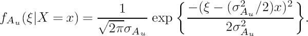
where f Au (ξ|X = x) is the conditional probability density function associated with the a priori LLR Au, and the information bits X are assumed to be equiprobable; i.e., we have P(X =+1) = P(X = −1) = 1/2.
In order to compute the mutual information I(X; Au) of Equation (4.12), the conditional PDF f Au(ξ|X = x) of the LLR Au has to be known. If we model the a priori LLR Au as an independent Gaussian random variable nAu having a variance of σ2 and a mean of zero in conjunction with the information bit X, then we have
where µAu must fulfill
According to the consistency condition [77] of LLR distribution, f Au(ξ|X = x)= f Au(−ξ|X = x) · exξξ and the conditional PDF fAu(ξ|X = x) becomes
Consequently, the mutual information IAu ![]() I(X; Au) defined in Equation (4.12) can be expressed as
I(X; Au) defined in Equation (4.12) can be expressed as

For the sake of notational compactness we define
Similarly, the same Gaussian model can be applied to the a priori LLR Ac, yielding
where µA c = σ2Ac/2 [98], and nA cis a Gaussian random variable with a variance of σ2 Ac and a mean of zero. Then, the mutual information between the encoded bit Y and the a priori LLR Ac can be expressed as

or in terms of the function J (·) as
The mutual information is also used to quantify the relationship of the extrinsic output IEu ![]() I(X; Eu) and IEc
I(X; Eu) and IEc ![]() I(Y ; Ec) with the original information bits and the encoded bits as follows:
I(Y ; Ec) with the original information bits and the encoded bits as follows:


4.2.2.2 Properties of the J (·) Function
The function J(·) defined in Equation (4.17) is useful for determining the mutual information. Hence we list some of its properties below.
- It is monotonically increasing, and thus it has a unique and unambiguous inverse function [98]
- Its range is [0 ...1] and it satisfies [98]
- The capacity CG of a binary input/continuous output AWGN channel is given by [98]
where σ2n is the variance of the Gaussian noise.
- · It is infeasible to express J(·) or its inverse in closed form. However, they can be closely approximated by [122]
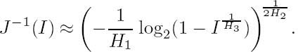
Numerical optimization to minimize the total squared difference between Equation (4.17) and Equation (4.26) results in the parameter values of H1 = 0.3073, H2 = 0.8935 and H3 = 1.1064. The solid curve in Figure 4.9 shows the values of Equation (4.17) and its visibly indistinguishable approximation in Equation (4.26).
4.2.2.3 Evaluation of the EXIT Characteristics of a SISO APP Module
According to the SISO APP algorithm outlined in Section 4.2.1, the extrinsic outputs Eu and Ec of a SISO APP module depend entirely on the a priori input Au and Ac. Hence the mutual information IEu or IEc quantifying the extrinsic output is a function of the mutual information IAu and IAc quantifying the a priori input, which can be defined as
Figure 4.9: The J(·) function of Equation (4.17) and its visibly indistinguishable approximation by Equation (4.26).

Figure 4.10: Figure 4.10: An EXIT module defined by two EXIT functions (4.28) and (4.29) of the corresponding SISO APP module.

These two functions are often referred to as the EXIT characteristics of a SISO module, since they characterize the SISO module’s capability of enhancing our confidence in its input information. Consequently, we can define an EXIT module, which is the counterpart of the corresponding SISO APP module in terms of mutual information transfer. Therefore the EXIT module has two inputs, namely, IAu and IAc as well as two outputs, namely, IEu and IEc, as depicted in Figure 4.10. The relationships between the inputs and the outputs are determined by the EXIT functions of Equation (4.28) and (4.29).
For simple codes such as repetition codes or single parity check codes, analytical forms of the associated EXIT characteristics may be derived. However, for the SISO modules of sophisticated codecs, their EXIT characteristics have to be obtained by simulation. In other words, for given values of IAu and IAc we artificially generate the a priori inputs Au and Ac, which are fed to the SISO module. Then the SISO APP algorithm of Section 4.2.1 is invoked, resulting in the extrinsic outputs Eu and Ec. Finally, we evaluate the mutual information IEu and IEc of Equation (4.21) and (4.22). In this way, the EXIT characteristics can be determined once a sufficiently high number of data points are accumulated. The detailed procedure is shown in Algorithm 4.2.
This is the original method proposed in [98] for the evaluation of the EXIT characteristics. Actually, Step 4 in Algorithm 4.2 may be significantly simplified [132, 259], as long as the outputs Eu and Ec of the SISO module are true a posteriori LLRs. In fact, the mutual information can be expressed as the expectation of a function of solely the absolute values of the a posteriori LLRs [132]. This result provides a simple method for computing the mutual information by simulation. Unlike the original method [98], it does not require explicit measurements of histograms of the soft outputs. More details are given below.
|
1) For given a priori input (IAu, IAc), compute the noise variance σ2Au and σ2Ac of the Gaussian model of Equation (4.13) using the inverse of the J(·) function, i.e. σAu = J−1(IAu) and σAc = J−1(IAc). 2) Generate a random binary sequence X with equally distributed values of { + 1, −1} and encode it, resulting in the encoded bit sequence Y. Then generate the a priori inputs Au and Ac using the Gaussian model of Equation (4.13), i.e. by scaling the input and adding Gaussian noise, where the noise variances are those obtained in Step 1. 3) Invoke the SISO APP algorithm to compute the extrinsic output Eu and Ec. 4) Use a histogram-based estimate of the conditional PDFs of fEu(ξ|Y = y) and fEc(ξ| Y =y) in Equation (4.21) and Equation (4.22) respectively. Then IEc compute the mutual information IEu and IEc according to Equation (4.21) and Equation (4.22) respectively. 5) Set IAu = IAu + Δ IAu, 0 ≤ IAu ≤ and IAc = IAc + Δ IAc, 0 ≤ IAc ≤ 1. Repeat Steps 1–4 until a sufficiently high number of data points are accumulated. |
4.2.2.4 Simplified Computation of Mutual Information
Let us first consider the mutual information I(Xn; Eu,n) between the a posteriori LLR Eu,n and the transmitted bit Xn, which can be expressed as
where E{x} denotes the expected value of x. In tangible physical terms Equation (4.30) quantifies the extra information gleaned with the advent of the knowledge of Eu,n. Note that, according to the definition of LLRs, the a posteriori probability P(Xn = ±1|λn) can be computed from the a posteriori LLR Eu,n =λn as P(Xn =±1|λn) = 1λn ![]() [70, 97]. Hence the conditional entropy H(Xn|Eu,n = λn) can be obtained as
[70, 97]. Hence the conditional entropy H(Xn|Eu,n = λn) can be obtained as

Therefore, the symbol-wise mutual information I(Xn; Eu,n) of Equation (4.30) may be expressed as
Similarly, we obtain the symbol-wise mutual information I(Yn; Ec,n) as
Consequently, the average mutual information IEu and IEc can be expressed as

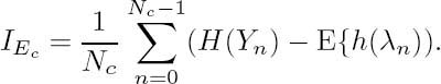
In general, both the input and the output bit values Xn and Yn are equiprobable; hence H(Xn) = H (Yn) = 1. Then Equations (4.36) and (4.37) may be simplified to


where fI(·) is
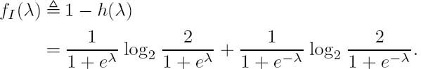
Assume furthermore that the a posteriori LLRs are ergodic and the block length is sufficiently high. Then the expectation values in Equation (4.38) and (4.39) can be replaced by the time averages [132,259]


The method outlined in Equations (4.41) and (4.42) has the following advantages.
- No LLR histograms have to be recorded; hence the computational complexity is significantly reduced. This method can operate ‘on-line,’ because as soon as a new a posteriori LLR becomes available it can be used to update the current estimate of the mutual information.
- The results are unbiased even for codes with time-varying trellises such as punctured convolutional codes, and bits having different statistical properties do not have to be treated differently [132].
Figure 4.11:EXIT function for CC(7,5) used as Decoder II in Figure 4.3.

4.2.2.5 Examples
In this section we will show examples of various EXIT functions that belong to different SISO modules. They are evaluated using the procedure outlined in Section 4.2.2.3. In general, a SISO module needs two EXIT functions (Equations 4.28) and (4.29) in order to characterize its information transfer behavior in iterative processing, for example when it is used as the intermediate decoder in multiple serial concatenation of component decoders. However, some of the input/output terminals of a SISO module may not be actively exploited in the iterative processing; hence, the employment of a single EXIT function may be sufficient on some occasions. We will discuss these scenarios separately in our forthcoming discourse.
4.2.2.5.1 The Intermediate Code. This is the general case. As seen from Figure 4.3, the intermediate SISO decoder receives its a priori input of IAc from the preceding SISO decoder, while its a priori input of IAu comes from the successive decoder. Correspondingly, it feeds back the extrinsic outputs of IEc and IEu respectively to the other two constituent decoders, as seen in Figure 4.3. Therefore, the pair of 2D EXIT functions described by Equations 4.28) and (4.29) are needed; these may be depicted in two 3D charts. For example, we show the two 2D EXIT functions of a half-rate convolutional code having the octal generator polynomials of (7, 5) in Figure 4.11.
4.2.2.5.2 The Inner Code. Some SISO modules, such as soft demappers (used, for example, in [84]) and SISO equalizers operate directly on channel observations. These SISO modules receive the a priori input IAu from the successive SISO module and feed back the extrinsic output IEu as seen in Figure 4.2. The input terminal IAc and the output terminal IE c are not used. Hence only a single EXIT function is needed. Moreover, the extrinsic output IE u also depends on the channel input; hence, IEu is usually expressed as a function of IAu
Figure 4.12: The EXIT functions of inner codes exemplified in Figure 4.2. The half-rate RSC code having octal generator polynomials of (5/7) and the half-rate NSC code having the octal generator polynomials of (7, 5) are used.

combined with Es/N0 as a parameter, i.e. we have
When using BPSK modulation, the EXIT function of the SISO decoder that is connected to the soft demapper, as exemplified in Figure 4.2, may also be characterized by Equation (4.43), since no iterative processing between the demapper and the decoder is needed. For example, we depict the EXIT functions of a half-rate Recursive Systematic Convolutional (RSC) code having octal generator polynomials of (5/7) and those of a half-rate Non-Systematic Convolutional (NSC) code using the same generator polynomials at several Es/N0 values in Figure 4.12. It can be seen that the EXIT functions of the RSC code always satisfy the condition of Tu (IAu = 1, Es/N0) = 1, while the EXIT functions of the NSC code do not.
4.2.2.5.3 The OuterCode. For SISO modules which are in the ‘outer’ positions of the concatenated scheme exemplified in Figure 4.2, the resultant EXIT functions may also be simplified to One-Dimensional (1D) functions. Since the input terminal IAu and the output terminal IEu are not used in the associated iterative processing, the EXIT function of an outer SISO module can be expressed as
Figure 4.13: The EXIT functions of various outer rate-1/2 non-recursive NSC decoders, where (g0, g1) represent the octal generator polynomials.

Figure 4.13 shows the EXIT functions of various non-recursive NSC codes used as outer codes. According to our informal observations, the RSC codes using the same generator polynomials have the same EXIT functions as the corresponding NSC codes.
4.3 Iterative Source–Channel Decoding Over AWGN Channels
This section investigates the performance of iterative source–channel decoding techniques. In general, channel coding is invoked after source coding for the sake of protecting the source information against the noise and other sources of impairments imposed by the transmission channel. In an approach inspired by the iterative decoding philosophy of turbo codes [69], the source code and channel code together may be viewed as a serially concatenated code [71], which can be decoded jointly and iteratively, provided that both the source decoder and the channel decoder are soft-in and soft-out components [42]. The performance of the iterative receiver is evaluated for transmission over AWGN channels, and the EXIT chart technique [98] is employed for analyzing the performance of iterative decoding and to assist in the design of efficient systems. Let us first introduce our system model.
4.3.1 System Model
The schematic diagram of the transmission system considered is shown in Figure 4.14. At the transmitter side of Figure 4.14, the non-binary source {uk} represents a typical source in a video, image or text compression system. It is modeled as a discrete memoryless source using a finite alphabet of {a1, a2 , ..., as}. The output symbols of the source are encoded by a source encoder, which outputs a binary sequence {bk}. We assume that the source encoder is a simple entropy encoder, which employs a Huffman code [9], RVLC [12] or VLEC [29] code. As shown in Figure 4.14, after interleaving the source-encoded bit stream is protected by an inner channel code against channel impairments. To be more specific, the inner code we employ is a convolutional code. Note that the interleaver seen in Figure 4.14 is used for mitigating the dependencies among the consecutive extrinsic LLRs in order to produce independent a priori LLRs. This is necessary because the independence of the a priori LLRs is assumed when the SISO APP algorithm multiplies the corresponding bit value probabilities in order to obtain their joint probabilities. The interleaver’s ability to achieve this goal is commensurate with its length and depends on how well its design facilitates ‘randomize’ the order of the LLRs.
Figure 4.14: Iteratively detected source and channel coding scheme.

At the receiver side of Figure 4.14, an iterative source–channel decoding structure is invoked, as in [42]. The iterative receiver consists of an inner APP channel decoder and an outer APP source decoder. Both of them employ the SISO APP module described in Section 4.2.1 and exchange LLRs as their reliability information.
The first stage of an iteration is constituted by the APP channel decoder. The input of the channel decoder is the channel output zk and the a priori information LA(xk) provided by the outer VLC decoder, which is LA(xk) = 0 for the first iteration. Based on these two inputs, the channel decoder computes the a posteriori information L (xk) and only the extrinsic information LE(xk) = L(xk)− LA(xk) is forwarded to the outer VLC decoder.
The second stage of an iteration is constituted by the bit-level trellis-based APP VLC decoder, which accepts as its input the a priori information LA(bk) from the inner channel decoder and generates the a posteriori information L(bk). Similarly, only the extrinsic information L(bk) = L(bk) − LA(bk) is fed back to the inner channel decoder. After the last iteration the source sequence estimation based on the same trellis, namely on that of the APP VLC decoder, is invoked in order to obtain the decoded source symbol sequence. Generally, the symbols of the non-binary source have a non-uniform distribution, which may be interpreted as a priori information. In order to be able to exploit this a priori source information, the APP algorithm of the SISO module has to be appropriately adapted, as detailed in Appendix B.
4.3.2 EXIT Characteristics of VLCs
We evaluated the associated EXIT characteristics for the various VLCs listed in Table 4.1. The corresponding results are depicted in Figure 4.15.
It can be seen in the figure that for the Huffman code the SISO VLC decoder only marginally benefits from having extrinsic information, even if exact a priori information is provided in the form of IA = 1. Upon increasing the code’s redundancy, i.e. decreasing the code rate, the SISO VLC decoder benefits from more extrinsic information, as observed for the RVLC-1, RVLC-2 and VLEC-3 schemes of Table 4.1; this indicates that higher iteration gain will be obtained when using iterative decoding. It is also worth noting that for VLCs having a free distance of df ≥ 2, such as the RVLC-2 and VLEC-3 schemes, the condition of T (IA = 1) = 1is satisfied. In contrast, for those having df = 1this condition is not satisfied, which indicates that a considerable number of residual errors will persist in the decoder’s output even in the high SNR areas. Note also that the starting point of the VLC EXIT function at the abscissa value of IA = 0is given by T (IA = 0) = 1− Hb , where Hb is the entropy of the VLC-encoded bits, which typically approaches one, giving a very low EXIT function starting point.
Table 4.1: VLCs used in the simulations

Figure 4.15: EXIT characteristics of VLCs listed in Table 4.1.

4.3.3 Simulation Results for AWGN Channels
In this section we present some simulation results for the proposed transmission scheme. All simulations were performed for BPSK modulation when communicating over an AWGN channel. The channel code used is a terminated memory-2, rate-1/2 RSC code having the generator polynomial of (g1/g0)8 =(5/7)8, where g0 is the feedback polynomial. For every simulation, 1000 different frames of length K = 1000 source symbols were encoded and transmitted. For the iterative receiver, six decoding iterations were executed, except for the Huffman code, where only three iterations were performed. The simulations were terminated either when all the frames were transmitted or when the number of detected source symbol errors reached 1000.
For the source encoder we use the VLCs as listed in Table 4.1. Since these codes have different rates, for the sake of fair comparison the associated Eb/N0 values have to be scaled by both the source code rate Rs and the channel code rate Rc as follows:
or in terms of decibels
where Es is the transmitted energy per modulated symbol, and M is the number of signals in the signal space of M -ary modulation. For example, M = 2 for BPSK modulation. The effect of the tail bits of the channel code is ignored here.
For every VLC, the transfer functions of the outer VLC decoder and the inner channel decoder are plotted in the form of EXIT charts in order to predict the performances of the iterative receivers.
The EXIT chart of the iterative receiver using the Huffman code of Table 4.1 and the corresponding SER performance are depicted in Figures 4.16 and 4.17 respectively. In the EXIT chart the transfer functions of the inner RSC decoder recorded at Eb/N0 = 0 dB, 1 dB and 2 dB are plotted. Moreover, the extrinsic information outputs, IEVLC and IERSC , of both decoders were recorded during our simulations and the average values at each iteration were plotted in the EXIT chart, which form the so-called decoding trajectories. The iterative decoding algorithm may possibly converge to a near-zero BER, when the decoding trajectory approaches the point (IA = 1, IE = 1). However, it can be readily seen that since the outer Huffman code has a flat transfer characteristic, it provides only limited extrinsic information for the inner channel decoder; hence, the overall performance can hardly be improved by iterative decoding. This is confirmed by the SER performance seen in Figure 4.17, where only a modest iteration gain is attained.
For the transmission scheme employing the RVLC-1 arrangement of Table 4.1, the iterative receiver did exhibit some iteration gain, as shown in Figure 4.19. However, the achievable improvements saturated after I = 2 or 3 iterations. This is because the two EXIT curves intersect, before reaching the (IA = 1, IE = 1) point, as shown in the EXIT chart of Figure 4.18, and the trajectories get trapped at these intersect points; hence, no more iteration gain can be obtained.
Figure 4.16: EXIT chart for the iterative receiver of Figure 4.14 using a Huffman code having df = 1 of Table 4.1 as the outer code and the RSC(2, 1, 2) code as the inner code for transmission over AWGN channels.

Figure 4.17: SER performance of the iterative receiver of Figure 4.14 using a Huffman code of Table 4.1 as the outer code and the RSC(2, 1, 2) code as the inner code for transmission over AWGN channels.

As already stated, the VLCs having df ≥ 2 exhibit better transfer characteristics, and hence also better convergence properties. This is confirmed in Figure 4.21, where the SER of the system employing the RVLC-2 scheme of Table 4.1 was continuously reduced for up to six iterations. At SER = 10−4, the iteration gain is as high as about 2.5 dB. As seen from the EXIT chart of Figure 4.20, for Eb/N0 > 1dB there will be an open EXIT ‘tunnel’ between the curves of the two transfer functions. This implies that if enough decoding iterations are performed, the iterative decoding trajectory will reach the (IA = 1, IE = 1) point of the EXIT chart, which is associated with achieving a near-zero BER. Note, however, that this will be only be possible if the iterative decoding trajectory follows the EXIT functions sufficiently well. This requires that the interleaver is sufficiently long and well designed in order for it to successfully mitigate the dependencies between the consecutive a priori LLRs, as described in Section 4.3.1.
Figure 4.18: EXIT chart for the iterative receiver of Figure 4.14 using a RVLC having df = 1 of Table 4.1 as the outer code and the RSC(2, 1, 2) code as the inner code for transmission over AWGN channels.

Figure 19.4: SER performance of the iterative receiver of Figure 4.14 using a RVLC having df of Table 4.1 as the outer code and the RSC(2, 1, 2) code as the inner code for transmission over AWGN channels.

Figure 4.20: EXIT chart for the iterative receiver of Figure 4.14 using a RVLC having df = 2 of Table 4.1 as the outer code and the RSC(2, 1, 2) code as the inner code for transmission over AWGN channels.

In the corresponding SER chart of Figure 4.21, the SER curve approaches the so-called ‘waterfall’ region or ‘turbo cliff’ region beyond this point. Hence, this Eb/N0 value is also referred to as the convergence threshold. It can also be seen from the EXIT chart of Figure 4.20 that, beyond the convergence threshold, the EXIT ‘tunnel’ between the two curves becomes narrow towards the top right corner near the point IA = 1, IE = 1. This indicates that the iteration gains will become lower during the course of iterative decoding. In particular, in the case of a limited interleaver size and for a low number of iterations a considerable number of residual errors will persist at the decoder’s output, and an error floor will appear even in the high channel SNR region.
Figures 4.22 and 4.23 show the EXIT chart and the SER performance of the system respectively, when employing the VLEC-3 scheme of Table 4.1. The convergence threshold of this system is about Eb/N0 = 0dB. Hence, beyond this point a significant iteration gain was obtained, as a benefit of the excellent transfer characteristics of the VLEC-3 code.
Figure 4.21: SER performance of the iterative receiver of Figure 4.14 using a RVLC having df = 2 of Table 4.1 as the outer code and the RSC(2, 1, 2) code as the inner code for transmission over AWGN channels.

At SER = 10−4, the achievable Eb/N0 gain is about 4 dB after six iterations and no error floor is observed. A performance comparison of the systems employing different VLCs is depicted in Figure 4.24. Clearly, in the context of iterative decoding, when the inner code is fixed, the achievable system performance is determined by the free distance of the outer code. The VLEC code having a free distance of df = 3 performs best after I = 6 iterations, while it has the lowest code rate and hence results in the lowest achievable system throughput. Similarly, the RVLC-2 scheme having df = 2 also outperforms the RVLC-1 having df = 1 and the Huffman code.
4.4 Iterative Channel Equalization, Channel Decoding and Source Decoding
In practical communications environments, the same signal may reach the receiver via multiple paths, as a result of scattering, diffraction and reflections. In simple terms, if all the significant multipath signals reach the receiver within a fraction of the duration of a single transmitted symbol, they result in non-dispersive fading, whereby occasionally they add destructively, resulting in a low received signal amplitude. However, if the arrival time difference among the multipath signals is higher than the symbol duration, then the received signal inflicts dispersive time-domain fading, yielding Inter-Symbol Interference (ISI).
The fading channel hence typically inflicts bursts of transmission errors, and the effects of these errors may be mitigated by adding redundancy to the transmitted signal in the form of error-correction coding, such as convolutional coding, as discussed in the previous section. However, adding redundancy reduces the effective throughput perceived by the end user. Furthermore, if the multipath signals are spread over multiple symbols they tend to further increase the error rate experienced, unless a channel equalizer is used. The channel equalizer collects all the delayed and faded multipath replicas, and linearly or nonlinearly combines them [260]. The equalizers typically achieve a diversity gain, because, even if one of the signal paths becomes severely faded, the receiver may still be able to extract sufficient energy from the other independently faded paths.
Figure 4.22: EXIT chart for the iterative receiver of Figure 4.14 using a VLEC code having df = 3 of Table 4.1 as the outer code and the RSC(2, 1, 2) code as the inner code for transmission over AWGN channels.

Figure 4.23: SER performance of the iterative receiver of Figure 4.14 using a VLEC code having df = 3 of Table 4.1 as the outer code and the RSC(2, 1, 2) code as the inner code for transmission over AWGN channels.

Figure 4.24: Performance comparison of the schemes employing different VLCs including Huffman code, RVLC-1 having df = 1, RVLC-2 having df = 2 and VLEC-3 having df = 3 of Table 4.1, after the first and the sixth iterations.

Capitalizing on the impressive performance gains of turbo codes, turbo equalization [82, 113, 261] has been proposed as a combined iterative channel equalization and channel decoding technique that has the potential of achieving equally impressive performance gains when communicating over ISI-contaminated channels. The turbo-equalization scheme introduced by Douillard et al. [82] may be viewed as an extension of the turbo decoding algorithm [69], which interprets the information spreading effects of the ISI as another form of error protection, reminiscent of that imposed by a rate-1 convolutional code. To elaborate a little further, the impulse response of the dispersive channel has the effect of smearing each transmitted symbol over a number of consecutive symbols. This action is similar to that of a convolutional encoder.
By applying the turbo detection principle of exchanging extrinsic information between channel equalization and source decoding, the receiver becomes capable of efficiently combatting the effects of ISI. In the following sections we describe such a scheme, where the redundancy inherent in the source is exploited for the sake of eliminating the channel-induced ISI. Transmission schemes both with and without channel coding are considered.
4.4.1 Channel Model
We assume having a coherent symbol-spaced receiver benefiting from the perfect knowledge of the signal’s phase and symbol timing, so that the transmit filter, the channel and the receiver filter can be jointly represented by a discrete-time linear filter having a finite-length impulse
Figure 4.25: Two dispersive Channel Impulse Responses (CIRs) and their frequency-domain representations.

response expressed as

where the real-valued channel coefficients {hm} are assumed to be time-invariant and known to the receiver. Figure 4.25 shows two examples of ISI-contaminated dispersive channels and their frequency domain responses introduced in [8]. The channel characterized in the upper two graphs is a three-path channel having moderate ISI, while the channel depicted in the lower two is a five-path channel suffering from severe ISI.
Given the Channel Impulse Response (CIR) of Equation (4.47) and a BPSK modulator, the channel output yk , which is also the equalizer’s input, is given by

Figure 4.26: Tapped delay line circuit of the channel model Equation (4.48) for M = 2.

where nk is the zero-mean AWGN having a variance of σ2. We assume that we have Nc = Nb + Nh , where Nh represents the so-called tailing bits concatenated by the transmitter, in order to take into account the effect of ISI-induced delay. More specifically, Nh = M number of binary zeros may be appended at the tail of an Nb-bit message, so that the discrete-time linear filter’s buffer content converges to the all-zero state. Explicitly, the channel’s output samples yk obey a conditional Gaussian distribution having a PDF expressed as

Figure 4.26 shows a tapped delay line model of the equivalent discrete-time channel of Equation (4.48) for M = 2, associated with the channel coefficients of h0 = 0.407, h1 = 0.815 and h2 = 0.407. Assuming an impulse response length of (M + 1), the tapped delay line model contains M delay elements. Hence, given a binary input alphabet of {+ 1, −1} , the channel can be in one of 2Mstates qi, i = 1, 2,. .. ,2M, corresponding to the 2M different possible binary contents in the delay elements. Let us denote the set of possible states by S = {q1, q2 ,..., q2M}. At each time instance of k = 1, 2, ..., Nc the state of the channel is a random variable sk ∈ S. More explicitly, we define sk =(dk, dk−1, ..., dk−M+ 1). Note that, given sk , the next state sk + 1 can only assume one of the two values determined by a + 1 or a −1 being fed into the tapped delay line model at time k + 1. The possible evolution of states can thus be described in the form of trellis diagram. Any path through the trellis corresponds to a sequence of input and output symbols read from the trellis branch labels, where the channel’s output symbol νk at time instance k is the noise-free output of the channel model of Equation (4.48) given by

The trellis constructed for the channel of Figure 4.26 is depicted in Figure 4.27. A branch of the trellis is a four-tuple (i, j, di,j, νi,j) , where the state sk+1 = qj at time k + 1can be reached from state sk =qi at time k , when the channel encounters the input dk =di,j and produces the output νk =νi,j , where di,j and νi,j are uniquely identified by the index pair (i, j). The set of all index pairs (i, j) corresponding to valid branches is denoted as B. For the
Figure 4.27: Trellis representation of the channel seen in Figure 4.26. The states q0 = (1, 1), q1 = (–1, 1), q2 = (1, –1), q3 = (–1, –1) are the possible contents of the delay elements in Figure 4.26. The transitions from a state sk = qi at time k to a state sk+1 = qj at time k + 1 are labeled with the input/output pair di,j/νi,j.

trellis seen in Figure 4.27, the set ![]() is as follows:
is as follows:
4.4.2 Iterative Channel Equalization and Source Decoding
In this section we investigate the principles of iterative equalization as well as source decoding, and derive the extrinsic information exchanged between the equalizer and the source decoder. We assume that the channel is an ISI-contaminated Gaussian channel, as expressed in Equation (4.48).
4.4.2.1 System Model
At the transmitter side, the output symbols of the non-binary source {xn} seen in Figure 4.28 are forwarded to an entropy encoder, which outputs a binary sequence {bk} , k = 1, 2,..., Nb. The source code used in the entropy encoder may be a Huffman code, RVLC [12] or VLEC code [29]. Then the resultant binary sequence is interleaved and transmitted over an ISI-contaminated channel also imposing AWGN, as shown in Figure 4.28.
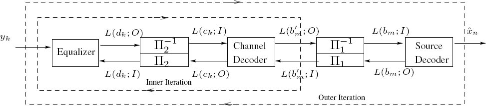
The receiver structure performing iterative equalization and source decoding is shown in Figure 4.29. The ultimate objective of the receiver is to provide estimates of the source symbols {xn}, given the channel output samples y ![]() y1Nc, where we have y1Nc {y1, y2 , ..., yNc}. More specifically, in the receiver structure of Figure 4.29 the channel equalizer’s feed-forward information generated in the context of each received data bit is applied to the source decoder through a deinterleaver described by the turbo deinterleaver function Π−1. The information conveyed along the feed-forward path is described by Lf (). In contrast, the source decoder feeds back the a priori information associated with each data bit to the channel equalizer through a turbo interleaver having the interleaving function
y1Nc, where we have y1Nc {y1, y2 , ..., yNc}. More specifically, in the receiver structure of Figure 4.29 the channel equalizer’s feed-forward information generated in the context of each received data bit is applied to the source decoder through a deinterleaver described by the turbo deinterleaver function Π−1. The information conveyed along the feed-forward path is described by Lf (). In contrast, the source decoder feeds back the a priori information associated with each data bit to the channel equalizer through a turbo interleaver having the interleaving function
Figure 4.28: Representation of a data transmission system including source coding and a turbo interleaver communicating over an ISI-channel inflicting additive white Gaussian noise.

Figure 4.29: Receiver schematic to perform iterative channel equalization and source decoding.

described by Π. The information conveyed along the feedback path is described by Lb(). This process is repeated for a number of times, until finally the source decoder computes the estimates {![]() n} for the source symbols {xn}, with the aid of the information provided by {Lf(bm)}. Let us first investigate the equalization process in a little more detail.
n} for the source symbols {xn}, with the aid of the information provided by {Lf(bm)}. Let us first investigate the equalization process in a little more detail.
4.4.2.2 EXIT Characteristics of Channel Equalizer
The channel equalization considered here is based on the APP algorithm, which makes the equalizer another manifestation of the SISO APP module described in Section 4.2.1. More details of the APP channel equalization can be found in Appendix C. Let us now study the transfer characteristics of the channel equalizer. Consider two ISI channels, namely the three-path and five-path CIRs depicted in Figure 4.25, which are represented by their CIR taps as
Figure 4.30 shows the EXIT functions of the channel equalizer for the dispersive AWGN channels of Equations (4.52) and (4.53) at different channel SNRs. It can be seen that the channel equalizer has the following transfer characteristics.
Figure 4.30: EXIT functions of the channel equalizer for transmission over the dispersive AWGN channels of Equations (4.52) and (4.53).

- The EXIT curves are almost straight lines, and those recorded for the same channel at different SNRs are almost parallel to each other.
- At low SNRs, IE = T(IA = 1) can be significantly less than 1, and IE = T(IA = 1) will be close to 1 only at high SNRs. This indicates that a considerable number of residual errors will persist at the output of the channel equalizer at low to medium SNRs.
- Observe in Figure 4.30 that the channel equalizer generally provides less extrinsic information IE for the five-path channel H2 than for the three-path channel H1 at the same input a priori information IA , which predicts potentially worse BER performance. Interestingly, the transfer functions of the two equalizers almost merge at IA = 1, i.e. they have a similar value of T(IA = 1). This indicates that they would have the same BER performance bound provided that all ISI were eliminated.
4.4.2.3 Simulation Results
In this section we evaluate the SER performance of the iterative receiver. In the simulations we used the three-path channel of Equation (4.52) and the five-path channel of Equation (4.53). For the source encoder we employed two different VLCs, namely the RVLC-2 and VLEC-3 schemes listed in Table 4.1. The encoded data is permutated by a random bit interleaver of size L = 4096bits.
The SER was calculated by using Levenshtein distance [251] for the combined transceiver using a RVLC, which was depicted in Figure 4.31, when transmitting over the three-path ISI channel H1 of Equation (4.52) and over the five-path ISI channel H2 of Equation (4.53). The performance of the same system over a non-dispersive AWGN channel is also depicted as a best-case ‘bound.’ It can be seen in Figure 4.31 that the iterative equalization and source decoding procedure converges as the number of iterations increases. This behavior is similar to that of a turbo equalizer [82] and effectively reduces the detrimental effects of ISI after I = 4iterations, potentially approaching the non-dispersive AWGN channel’s performance.
Figure 4.31: SER performance of the RVLC-2 of Table 4.1 for transmission over the dispersive AWGN channels of Equation (4.52) and (4.53).

The SER performance of the system using a VLEC code of Table 4.1 is depicted in Figure 4.32, when transmitting over the three-path ISI channel H1 of Equation (4.52) and over the five-path ISI channel H2 of Equation (4.53). Since the VLEC code has a larger free distance, and hence a stronger error-correction capability, the iterative equalization and source decoding procedure succeeds in effectively eliminating the ISI, and approaches the non-dispersive AWGN performance bound after I = 4 iterations.
4.4.2.4 Performance Analysis Using EXIT Charts
In order to analyze the simulation results obtained, we measured the EXIT characteristics of the channel equalizer as well as those of the VLC decoder, and plotted their EXIT charts in Figure 4.33. Specifically, both the EXIT chart and the simulated decoding trajectory of the system using RVLC-2 of Table 4.1 for communicating over the three-path channel H1 are shown in Figure 4.33a. At Eb/N0 = 4 dB, the transfer function of the channel equalizer and that of the VLC decoder intersect in the middle, and after three iterations the trajectory becomes trapped, which implies that little iteration gain can be obtained, even if more iterations are executed. Upon increasing Eb/N0, the two transfer functions intersect at higher (IA , IE) points and the tunnel between the two EXIT curves becomes wider, which now indicates that higher iteration gains can be achieved, and hence the resultant SER becomes lower. Similar observations can be made from the EXIT chart of the same system communicating over the five-path channel H2 of Figure 4.33b, except that the channel equalizer needs an almost 3 dB higher Eb/N0 to obtain a similar transfer characteristic. Hence the SER curves are shifted to the right by almost 3 dB, as shown in Figure 4.31.
Figure 4.32: SER performance of the VLEC code of Table 4.1 for transmission over the dispersive AWGN channels of Equation (4.52) and (4.53).

Figure 4.33c shows the EXIT chart and the simulated decoding trajectory of the system using VLEC-3 of Table 4.1 for communicating over the three-path channel H1. Compared with the system using RVLC-2 (Figure 4.33a), there is a significantly wider tunnel between the two EXIT curves at the same Eb/N0; hence higher iteration gains can be obtained at a lower number of iterations. This is mainly the benefit of the significantly lower coding rate of the VLEC code used (RVLEC -3 = 0.54 < RRVLC -2 = 0.87). However, the system still suffers from a significant number of residual errors, since the two EXIT curves intersect in the middle and the resultant decoding trajectory gets trapped before reaching the top right corner of (IA = 1, IE = 1).
Figure 4.33d shows the EXIT chart and the actual decoding trajectory of the same system when communicating over the five-path channel H2. For the same Eb/N0, the equalizer communicating over the five-path channel has a steeper EXIT curve than for transmission over the three-path channel, and its initial point at (IEEQ = T(IAEQ = 0)) is significantly lower. After the first iteration, the extrinsic output of the VLEC decoder remains smaller. Hence the SER performance recorded after the first iteration is always worse than that of the system communicating over the three-path channel. At low Eb/N0 values (e. g. <4dB), the EXIT tunnel between the inner code’s curve and the outer code’s curve remains rather narrow. By contrast, at high Eb/N0 values (e. g. ≥ 6 dB), the tunnel becomes significantly wide and has almost the same extrinsic output as that recorded for the three-path channel (Figure 4.33c) after five iterations. Hence the SER performances of the system recorded over the three-path channel and the five-path channel converge at high Eb/N0 values, as shown in Figure 4.32.
Figure 4.33: EXIT charts of the channel equalizer as well as the VLC decoder and the actual decoding trajectories at various Eb/N0 values.

4.4.3 Precoding for Dispersive Channels
When the channel is non-recursive, which is the case for all wireless channels, then the gain of the iterative equalization remains limited. More explicitly, the performance of the outer channel code for transmission over AWGN channels represents an upper bound on the achievable receiver performance. In order to achieve a performance better than this, either the outer code can be replaced with a turbo code, as suggested in [262], or the channel can be made to appear recursive to the receiver, thus enabling us to achieve a higher interleaver gain. In the family of the latter techniques, recursive rate-one precoders, which effectively render the channel recursive, have been shown to yield significant performance gains in iterative equalization systems [263]. The concept was first presented in [105, 264, 265] for magnetic recording channels, and has subsequently been investigated in [263, 266] using BPSK modulations and in [212] using higher order modulations for general dispersive channels. A further advantage of the precoder is that there is no substantial increase in receiver complexity associated with its inclusion, as long as the memory of the precoder is no higher than that of the dispersive channel.
Figure 4.34: An example of precoding for BPSK modulation.
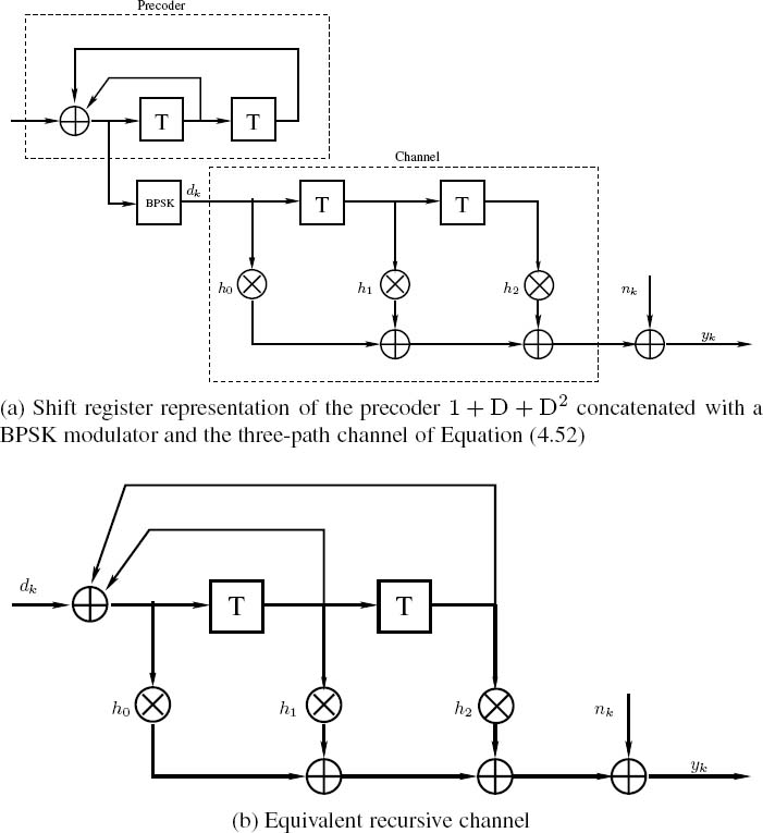
The precoder is generally described in terms of a shift register having feedback connections, described by a feedback polynomial. The structure is essentially the same as that of a recursive convolutional encoder. Figure 4.34 shows an example of a precoded channel.
4.4.3.1 EXIT Characteristics of Precoded Channel Equalizers
In this section we investigate the EXIT characteristics of precoded channel equalizers. Again, the three-path channel of Equation (4.52) and the five-path channel of Equation (4.53) are used as examples. For the three-path channel, the generator polynomials of the precoders having a memory of m ≤ 2 are 1 + D, 1 + D + D2 and 1 + D2. The EXIT functions of the operating channel equalizer both with and without these precoders for transmission over the three-path channel are shown in Figure 4.35a. It can be seen that, when using a precoder, the EXIT function can reach the (IA = 1, IE = 1) point, while this is not the case for the non-precoded system. Hence the channel equalizer is capable of achieving near error-free detection for transmission over precoded channels, while it encounters an error rate floor when communicating over non-precoded channels. Furthermore, all the EXIT functions recorded for precoded channels have lower initial values at (T (IA = 0)) in comparison with the non-precoded case, and this initial value decreases upon increasing the polynomial’s order.
Similarly, we study the EXIT function of the channel equalizer for transmission over the five-path channel. As the five-path channel has a memory of 4, there are a total of 15 different precoders having a memory of m ≤ 4. Only eight of them were selected for quantitative characterization in Figure 4.35b. Similar observations are obtained as in the case of the three-path channel, such as that the transfer functions arrive at the (IA = 1, IE = 1) point when using precoders as well as having lower start values.
4.4.3.2 Performance Analysis
The performance analysis of the joint channel equalization and source decoding system communicating over precoded channels is presented in this section. As observed in Section 4.4.3.1, precoders have similar effects to the channel equalizer’s EXIT characteristics in the case of both the three-path and the five-path channels. Hence, we only consider the three-path channel here, and the precoders used are (1 + D) and (1 + D2). For source coding we used the RVLC-2 and VLEC-3 schemes of Table 4.1. In all simulations, L = 1000 source symbols were encoded and transmitted in each frame.
First, the EXIT charts of the system using the RVLC-2 of Table 4.1 and precoder (1 + D) as well as (1 + D2) are depicted in Figures 4.36a and 4.36b respectively. As seen from Figure 4.36a, the transfer function of the inner channel equalizer and that of the outer source decoder intersect before reaching the (IA = 1, IE = 1) point. The coordinates of the intersection point increase upon increasing the channel SNR, until the (IA = 1, IE = 1) point is reached. Hence we can predict that for the system using the precoder (1 + D) the iteration gains will saturate after a certain number of iterations, and the achievable error rate is limited, which is similar to the case of non-precoded channels. In contrast, for the case of the precoder (1 + D2) different observations may be made. As seen from Figure 4.36b, Eb/N0 = 5.2dB is the system’s convergence threshold. Above this Eb/N0 value, the EXIT functions of the inner channel equalizer and the outer source decoder intersect only at the (IA = 1, IE = 1) point. Hence it is possible to achieve error-free detection provided that the interleaver length and the number of iterations are sufficiently high. Also shown in Figure 4.36 are the simulated decoding trajectories, which follow the EXIT chart predictions quite well. Further confirmations accrue from the simulated SER performances shown in Figure 4.37. For the system using the precoder (1 + D), the achievable SER is bounded by the performance when transmitting over an AWGN channel, as seen from Figure 4.37a. In contrast, for the system using the precoder (1 + D2), the SER can in fact outperform the bound and attain a lower value at high channel SNRs, as seen from Figure 4.37b, although it performs slightly worse in the low SNR region in comparison with the system using the precoder (1 + D), due to the lower extrinsic output of the equalizer previously observed in Figure 4.36.
Similarly, we analyze the achievable performances of the various systems using VLEC-3 of Table 4.1. The corresponding EXIT charts are shown in Figure 4.38. Both systems using the precoders (1 + D) and (1 + D2) show meritorious EXIT characteristics, where an open tunnel can be obtained between the two curves until the (IA = 1, IE = 1) point is reached.
Figure 4.35: EXIT functions of the APP equalizer for transmission over precoded dispersive AWGN channels.

Figure 4.36: EXIT charts of the channel equalizer and the VLC decoder using the RVLC-2 scheme of Table 4.1 over the precoded three-path channel of Equation (4.52).

Figure 4.37: SER performance of the iterative receiver using the RVLC-2 scheme of Table 4.1 for transmission over the precoded dispersive AWGN channel of Equation (4.52).
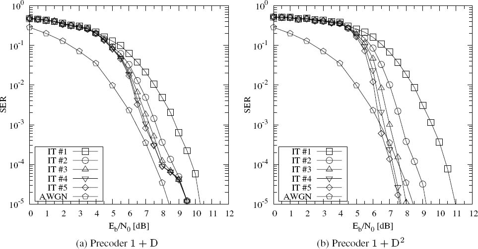
Furthermore, the system using the precoder (1 + D) has a lower convergence threshold of Eb/N0 = 2.1 dB than that using the precoder (1 + D2), which attains convergence at Eb/N0 = 2.8 dB. The corresponding SER performances are shown in Figure 4.39. Both systems can outperform the performance bounds of non-precoded systems. In particular, the system using the precoder (1 + D) benefits from earlier convergence and attains a SER of 10−4 at Eb/N0 = 3.6 dB, while the system using the precoder (1 + D2) needs Eb/N0 = 4.2 dB to achieve the same SER.
Figure 4.38: EXIT charts of the channel equalizer and the VLC decoder using the VLEC-3 scheme of Table 4.1 for transmission over the precoded three-path channel of Equation (4.52).

Figure 4.39: SER performance of the iterative receiver using the VLEC-3 scheme of Table 4.1 for transmission over the precoded three-path channel of Equation (4.52).

Figure 4.40: Transmitter schematic of the joint source-channel coding scheme for transmission over dispersive channels.

Figure 4.41: Receiver schematic of iterative channel equalization, channel decoding and source decoding.
4.4.4 Joint Turbo Equalization and Source Decoding
In this section we will investigate the achievable performance of iterative equalization, when both channel decoding and source decoding are considered, which constitutes a three-stage serially concatenated scheme. Let us first introduce our system model.
4.4.4.1 System Model
We assume that the source-encoded data is protected by a channel code before its transmission over an ISI-contaminated channel, as shown in Figure 4.40. At the receiver channel equalization, channel decoding and source decoding are performed iteratively. Generally, the iterative channel equalization and channel decoding processes, carried out in a two-stage structure, are referred to together as turbo equalization. However, when using SISO source decoding as well, the joint channel equalization, channel decoding and source decoding scheme of Figure 4.41 also becomes capable of exploiting the residual redundancy inherent in the source.
More explicitly, the corresponding receiver consists of three SISO modules, the channel equalizer, the channel decoder and the source decoder, as shown in Figure 4.41. All of them employ similar APP decoding algorithms and generate soft output for the benefit of the next processing stage. The channel equalization and channel decoding form the inner iterations. After a certain number of inner iterations, the source decoder is invoked and the extrinsic information of the source is fed back for the next inner iteration. During our experiments, we found that the activation of one outer iteration after two inner iterations offered a good trade-off between the complexity imposed and the achievable performance. At the last outer iteration the source decoder generates the estimate {![]() n} of the source symbol sequence by employing a sequence detection on the basis of the classic Viterbi algorithm using the same bit-level trellis.
n} of the source symbol sequence by employing a sequence detection on the basis of the classic Viterbi algorithm using the same bit-level trellis.
4.4.4.2 Simulation Results
The attainable performance of the amalgamated turbo receiver depicted in Figure 4.41 has been evaluated when communicating over the three-path ISI channel H1 of Equation (4.52). The channel code used here is a half-rate, constraint-length K = 5 RSC code, using the octally represented generator polynomial of G = (035/023). The source code used is the RVLC-2 scheme of Table 4.1. The two interleavers are random bit-interleavers having a memory of 2048 bits and 4096 bits respectively. These system parameters are also listed in Table 4.2.
The corresponding simulation results are depicted in Figure 4.42. The performances of both the joint and the separate source-decoding and turbo-equalization schemes are depicted. No outer iterations were executed in the separate source-decoding-based scheme. The performance of the same system for transmission over the non-dispersive AWGN channel after I = 6 iterations is also depicted as the best-case performance ‘bound.’ As we can observe in Figure 4.42, the joint three-stage turbo-detection scheme outperforms the separate source-decoding-based scheme by about 2 dB at SER = 10−4 after I = 6 iterations.
Table 4.2: System parameters used in the simulations

4.5 Summary and Conclusions
In this chapter the achievable performances of iterative source–channel decoding schemes were investigated for both non-dispersive and dispersive AWGN channels. Since a source decoder combined with a channel decoder or a channel equalizer may be viewed as a serially concatenated system, the design principle of serial concatenated codes [71] applies, where the free distance of the outer code predetermines the achievable interleaver gain.
Figure 4.42: SER performance of joint RVLC decoding, channel decoding and channel equalization over the three-path dispersive AWGN channel of Equation (4.52).

To be more specific, in the case of non-dispersive AWGN channels our simulation results show that the RVLC-2 of Table 4.1 having df = 2 outperforms the Huffman code and RVLC1having df = 1, while VLEC-3 having df = 3 outperforms the RVLC-2 arrangement. When the source codes have the same free distance, as with the Huffman code and RVLC-1 of Table 4.1, the constraint length determines the achievable performance. The larger the constraint length, the better the attainable performance. Our EXIT chart analysis seen in Figure 4.33 confirms the simulation results of Figures 4.37 and 4.39. It was found that VLCs having df ≥ 2, such as RVLC-2 and VLEC-3, have better convergence properties than their lower-free-distance counterparts.
Unlike those of convolutional codes, the free distance and the code rate of a source code cannot be adjusted separately. Increasing the free distance usually requires a decrease in the code rate. For example, as the free distance increases from 1 to 3, the code rate of the Huffman code, RVLC-1, RVLC-2 and VLEC-3 schemes decreases from 0.98 to 0.54. Increasing the free distance generally improves the attainable decoding performance. However, decreasing the code rate reduces the system’s throughput. For the design of the entire system, we have to find an attractive balance between the code rate and the free distance. Our main results are summarized in Table 4.3.
Furthermore, in the case of dispersive AWGN channels, the performance of iterative channel equalization and source decoding is evaluated for transmission over a three-path channel having mild ISI and a five-path channel having severe ISI. For both channels, the system using either the RVLC-2 or the VLEC-3 code of Table 4.1 exhibits significant iteration gains. Indeed, the EXIT chart analysis of Figure 4.30 shows that the EXIT function of a channel equalizer cannot reach the (IA = 1, IE = 1) point, except for high SNRs, which implies that residual errors persist at the channel equalizer’s output, regardless how high the interleaver length is and how many iterations are executed. This is further confirmed by the simulation results of Figures 4.31 and 4.32, where the performance of the iterative receiver is bounded by the performance of the same system transmitting over an AWGN channel exhibiting no ISI, resulting in ‘error shoulders’ in the SER curves. The system using the VLEC-3 code performs closer to the non-dispersive AWGN bound than that using the RVLC-2 due to the better EXIT characteristics of the VLEC-3 code.
TABLE 4.3: Summary of the simulation results for the iterative source–channel decoding scheme investigated in Section 4.3: various source codes listed in Table 4.1 are evaluated

†The system throughput is measured in bits per channel use (bpc).
‡The Eb/N0 gain is based on the SNR value required to achieve a SER of 10−4after six iterations, and the benchmark is the scheme using the Huffman code.
Table 4.4: Summary of the simulation results of the iterative source decoding and channel equalization scheme for transmission over the three-path channel H1 investigated in Section 4.4 – the RVLC-2 and the VLEC-3 code listed in Table 4.1 are employed, resulting in a system throughput of 0.87 bpc and 0.54 bpc respectively
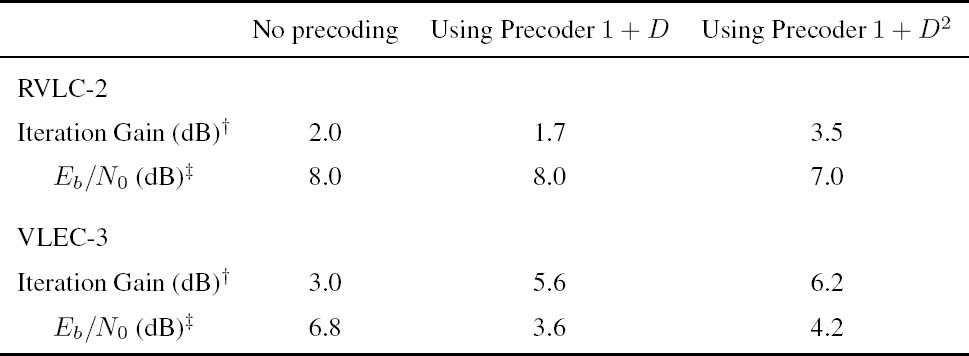
‡ The iteration gain is measured after five iterations.
‡ The Eb/N0 value is the SNR value required for achieving a SER of 10-4 after five iterations.
The effect of precoding on the iterative channel equalization and source decoding was also investigated. A rate-one precoder renders the channel recursive for the receiver, and thus enables the attainment of higher interleaver gains. This effect is more obvious in the EXIT chart analysis of Figure 4.35, where the EXIT function of a channel equalizer recorded for a precoded channel can reach the (IA = 1, IE = 1) point. It was found in Section 4.4.3 that for different source codes different precoders should be used. For example, when using RVLC-2, the system employing the precoder (1 + D) inflicts an error floor, while the system employing the precoder (1 + D2) does not. By contrast, when using VLEC-3, the system employing the precoder (1 + D) achieves earlier convergence than that employing the precoder (1 + D2), while both systems avoid having error floors. Therefore it is concluded that the source code and the precoder should be designed jointly. Our main findings are summarized in Table 4.4.
Finally, when a channel code is employed at the transmitter, a three-stage iterative receiver is formed consisting of a channel equalizer, a channel decoder and a source decoder. It was found in Figure 4.42 that up to 2 dB gain in terms of Eb/N0 values required for achieving a SER of 10−5 can be obtained, when compared with separate turbo equalization and source decoding.
1Parts of this chapter are based on the collaborative research outlined in [209]© IEEE (2005), and [210]© IEEE (2006).