
Chapter 5
Three-Stage Serially Concatenated Turbo Equalization1
5.1 Introduction
Turbo equalization [82] is an effective means of eliminating the channel-induced ISI imposed on the received signal. Hence, the achievable performance may approach that recorded over the non-dispersive AWGN channel, as detailed in [70] in the context of diverse turbo equalizers. When a simple rate-1 precoder is applied before the modulator, which renders the channel to appear recursive to the receiver, the attainable performance may be further improved [105, 263].
The SISO Minimum Mean Square Error (MMSE) equalizer [131], which is capable of utilizing a priori information from other SISO modules such as a SISO channel decoder, and generating extrinsic information, forms an attractive design alternative to the MAP equalizer owing to its lower computational complexity. This is particularly so for channels having long CIRs [113, 131]. The precoder can be readily integrated into the shift register model of the ISI channel [263], and may be modeled by combining its trellis with the trellis of a MAP/Soft-Output Viterbi Algorithm (SOVA)-based equalizer. However, the precoder’s trellis description cannot be directly combined with the model of a MMSE equalizer. Hence, the achievable performance of MMSE turbo equalization is potentially limited [113, 131].
EXIT [98] charts have been proposed for analyzing the convergence behavior of iterative decoding schemes, and indicate that an infinitesimally low BER may only be achieved by an iterative receiver if an open tunnel exists between the EXIT curves of the two SISO components. Recently, both the convergence analysis and the best activation order of the component codes has been studied in the context of multiple-stage concatenated codes [120, 122], which generally require the employment of three-dimensional (3D) EXIT charts. For the sake of simplifying the associated analysis, a 3D to 2D EXIT chart projection technique was proposed in [120, 122]. It has been shown [113] that the EXIT curve of a MMSE equalizer intersects with that of the channel decoder before reaching the decoding convergence point of (1,1); hence, residual errors persist after turbo equalization. However, it is natural to conjecture that there might exist an open tunnel leading to the convergence point in the 3D EXIT chart of a well-designed three-stage SISO system.
Against this backdrop, we propose a combined serially concatenated channel coding and MMSE equalization scheme, which is capable of achieving a precoding-aided convergence acceleration effect for a MAP/SOVA equalizer. Moreover, the convergence behavior of the proposed scheme is investigated with the aid of the 3D to 2D EXIT chart projection technique developed in [120, 122], and further design guidelines are derived from an EXIT-chart perspective. For illustration and comparison, let us commence with the family of traditional two-stage turbo equalization schemes.
5.2 Soft-In Soft-Out MMSE Equalization
We assume a coherent, symbol-spaced receiver front end as well as perfect knowledge of the signal phase and symbol timing, where the transmitter filter, the channel and the receiver filter are represented by a discrete-time linear filter having the Finite-length Impulse Response (FIR)
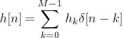
of length M. The coefficients hk are assumed to be time invariant and known to the receiver. For simplicity, we assume Binary Phase-Shift Keying (BPSK) and that the channel impulse response coefficients hk and the noise samples wn are real valued. For higher-order constellations and complex-valued hk and wn, please refer to [131] for the details.
Let xn, n = 1, ..., Kc, xn ∈ { + 1, − 1} denote the transmitted symbols and wn represent the AWGN samples, which are independent and identically distributed (i.i.d.). Given Equation (5.1), the receiver’s input zn is given by

Then the MMSE equalizer computes the estimates ![]() n of the transmitted symbols xn from the received symbols zn by minimizing the cost function E [|xn −
n of the transmitted symbols xn from the received symbols zn by minimizing the cost function E [|xn − ![]() n|2].
n|2].
In contrast with conventional MMSE-based equalization methods, in the SISO equalizer advocated the mean squared error is averaged over both the distribution of the noise and the distribution of the transmitted symbols. This is because, in contrast to classic MMSE-based non-iterative equalization, in the context of turbo equalization the symbol distribution is no longer i.i.d., as is typically assumed, due to the information fed back to the equalizer from the error-correction decoder. Let ![]() denote the a priori LLR provided by the channel decoder. Then the SISO equalizer’s output LE(xn) is obtained using the estimate
denote the a priori LLR provided by the channel decoder. Then the SISO equalizer’s output LE(xn) is obtained using the estimate ![]() n:
n:

n = 1, ..., Kc, which requires the knowledge of the distribution p(![]() n|xn = x).
n|xn = x).
In order to perform MMSE estimation, the statistics ![]() n
n ![]() E[xn] and vn
E[xn] and vn ![]() Cov(xn, xn) of the symbols xn are required. Usually, the symbols xn are assumed to be equiprobable and i.i.d., which corresponds to LA(xn) = 0, ∀n, and yields
Cov(xn, xn) of the symbols xn are required. Usually, the symbols xn are assumed to be equiprobable and i.i.d., which corresponds to LA(xn) = 0, ∀n, and yields ![]() n = 0 as well as vn = 1. For the general case of LA(xn) ∈
n = 0 as well as vn = 1. For the general case of LA(xn) ∈ ![]() , when the symbols xn are not equiprobable,
, when the symbols xn are not equiprobable, ![]() n and vn are obtained as
n and vn are obtained as


After MMSE estimation, we assume that the PDFs p(![]() n|xn = x) are Gaussian, having the parameters of µn, x
n|xn = x) are Gaussian, having the parameters of µn, x ![]() E[
E[![]() n|xn = x] and σ2n, x
n|xn = x] and σ2n, x ![]() Cov(
Cov(![]() n,
n, ![]() n|xn = x) [90]:
n|xn = x) [90]:
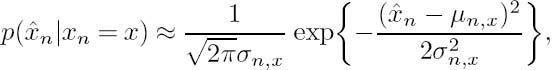
and the corresponding output LLRs LE(xn) are formulated as
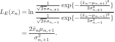
The employment of the Gaussian assumption tremendously simplifies the computation of the SISO equalizer output LLRs LE(xn). We emphasize that LE(xn) should not depend on the particular a priori LLR LA(xn). Therefore, we require that ![]() n does not depend on LA(xn), which affects the derivation of the MMSE equalization algorithms. For more details we refer to [113, 131].
n does not depend on LA(xn), which affects the derivation of the MMSE equalization algorithms. For more details we refer to [113, 131].
Figure 5.1: Turbo equalization system using MAP/MMSE equalizer both with and without precoding. The system parameters are summarized in Table 5.1.

5.3 Turbo Equalization Using MAP/MMSE Equalizers
5.3.1 System Model
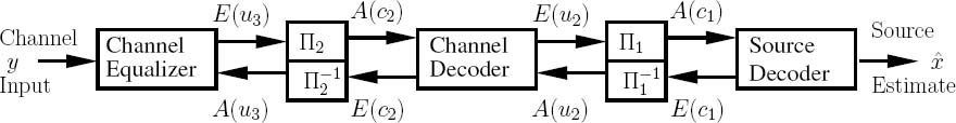
Figure 5.1 shows the system model of a classic turbo equalization scheme. At the transmitter, a block of length L information data bits u1 is first encoded by a channel encoder. After channel coding the coded bits c1 are interleaved, yielding the data bits u2, and they are either directly fed to the bit-to-modulated-symbol mapper or first fed through a rate-1 precoder and encoded to produce the coded bits c2, as seen in Figure 5.1. After mapping, the modulated signal x is transmitted over a dispersive channel contaminated by AWGN n. At the receiver of Figure 5.1, an iterative detection/decoding structure is employed, where extrinsic information is exchanged between the channel equalizer and the channel decoder in a number of consecutive iterations. To be specific, the channel equalizer processes two inputs, namely the received signal y and the a priori information A(u2) fed back by the channel decoder. Then the channel equalizer of Figure 5.1 generates the extrinsic information E(u2), which is deinterleaved and forwarded as the a priori information to the channel decoder. Furthermore, the channel decoder capitalizes on the a priori information A(c1) provided by the channel equalizer and generates the extrinsic information E(c1), which is interleaved and fed back to the channel equalizer as the a priori information. Following the last iteration, the estimates ![]() 1 of the original bits are generated by the channel decoder, as seen in Figure 5.1.
1 of the original bits are generated by the channel decoder, as seen in Figure 5.1.
In our forthcoming EXIT chart analysis and Monte Carlo simulations, we assume that the channel is time invariant and that the CIR is known at the receiver. To be specific, the three-path CIR of [8], described by
is used. We employ a constraint-length 3, half-rate RSC code RSC(2,1,3) having the octally represented generator polynomials of (5/7), where 7 is the feedback polynomial and 5 is the feed-forward polynomial. Then we use a simple rate-1 precoder described by the generator polynomials of 1/(1 + D). Either MAP or MMSE equalization is invoked, but precoding is only combined with the MAP equalizer. For the sake of simplicity, BPSK modulation is used. Our system parameters are summarized in Table 5.1.
5.3.2 EXIT Chart Analysis
Figure 5.2 depicts the EXIT functions of both the MAP/MMSE equalizers and the outer convolutional decoder. It is clear that the EXIT curves of both the MMSE equalizer and the MAP equalizer (without precoding) intersect with that of the outer RSC(2,1,3) decoder, before reaching the convergence point of (IEQA = 1, IEQE = 1). Hence residual errors may persist, regardless of both the number of iterations used and the size of the interleaver. Furthermore, the MMSE equalizer generally outputs less extrinsic information than the MAP equalizer does, resulting in a poorer performance. On the other hand, with the advent of precoding, the EXIT curve of the MAP equalizer becomes capable of reaching the convergence point, as seen in Figure 5.2. We note, however, that there is a crossover between the EXIT curves of the precoded and the non-precoded MAP equalizer, which implies that the non-precoded MAP equalizer would perform better in the low-SNR region, while the precoded MAP equalizer is capable of achieving an near error-free performance, provided that enough iterations are performed. The convergence threshold of the precoded MAP equalizer is about 2.3 dB.
Table 5.1: System parameters used in this section
| RSC(2,1,3) | |
| Channel encoder | Generator polynomials (5/7) |
| Precoder | Generator polynomials 1/(1 + D) |
| Modulation | BPSK |
| CIR | [0.407 0.815 0.407]T |
| Block length | L = 4096 bits |
5.3.3 Simulation Results
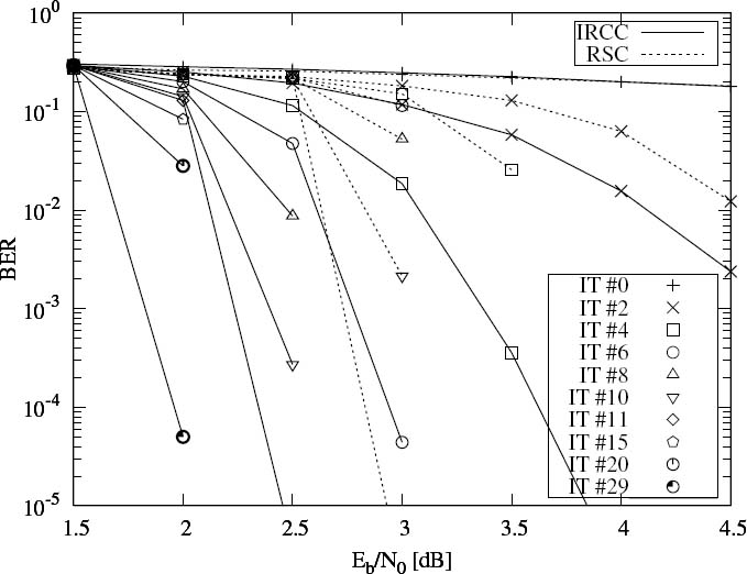
In order to verify the convergence prediction of the EXIT chart analysis outlined in Section 5.3.2, Monte Carlo simulations were also performed and the corresponding BER results are depicted in Figure 5.3. It can be seen that the BER performance of the precoded system becomes better than that of the non-precoded system at an Eb/N0 of about 2.7 dB.
5.4 Three-Stage Serially Concatenated Coding and MMSE Equalization
5.4.1 System Model
Simply incorporating an interleaver between the precoder and the signal mapper in the transmitter of Figure 5.1 enables the receiver to perform iterative equalization/decoding by exchanging extrinsic information between three SISO modules, namely the MMSE equalizer, Decoder II and Decoder I of Figure 5.4. Here, we would prefer not to refer to Encoder II as a precoder, since it cannot be directly combined with the equalizer at the receiver as in Figure 5.1. The same three-path channel of Equation (5.8) is used as in Section 5.3. The length of the non-causal and the causal parts of the MMSE filter are N1 = 5 and N2 = 3 respectively, resulting in an overall filter length of N = N1 + N2 + 1 = 9.
Figure 5.2: EXIT charts for the iterative receiver using either a MMSE equalizer or a MAP equalizer, where the latter is investigated for both a non-precoded and a precoded channel at Eb/N0 = 3dB.

5.4.2 EXIT Chart Analysis
In the following, we will carry out the EXIT chart analysis of the three-stage system of Figure 5.4. As with the two-stage system, the convergence SNR threshold of the three-stage system can be determined. At the same time, the outer code is optimized to give the lowest convergence SNR threshold. Finally, the activation order of the three SISO modules is optimized.
5.4.2.1 Determination of the Convergence Threshold
As seen in Figure 5.4, Decoder II exploits two a priori inputs, namely A(c2) and A(u2). At the same time, it generates two extrinsic outputs, E(c2) and E(u2). Hence, in order to describe the EXIT characteristics of Decoder II, we need the following two 2D EXIT functions [98, 122]:
In contrast, for the MMSE equalizer and Decoder I only one a priori input is available in Figure 5.4, and the corresponding EXIT functions are
Figure 5.3: BER performance of the iterative receiver using the MAP equalizer both with and without precoding, for transmission over the dispersive AWGN channel having a CIR of Equation (5.8). The system parameters are outlined in Table 5.1.

Figure 5.4: System diagram of two serially concatenated codes and MMSE equalization.

for the equalizer and
for Decoder I, where the second parameter, Eb/N0, in Equation (5.11) indicates that the extrinsic information also depends on the channel SNR. Therefore, with the aid of the EXIT module concept as described in Section 4.2.2, the three-stage system of Figure 5.4 may be viewed as a serial concatenation of three EXIT modules, which is shown in Figure 5.5.
In order to plot all of the EXIT functions, two 3D EXIT charts are required, namely one for the EXIT functions of both Equations (5.10) and (5.11) as shown in Figure 5.6a, and another for the EXIT functions of both Equations (5.9) and (5.12) as shown in Figure 5.6b. Note that IE(u3) of Equation (5.11) is independent of IA(u2); hence the MMSE equalizer’s EXIT surface seen in Figure 5.6a is generated by sliding its EXIT curve in the 2D EXIT chart of Figure 5.2 along the IA(u2) axis. The EXIT surface of Decoder I was generated similarly, as shown in Figure 5.6b, where IE(c1) of Equation (5.12) is independent of IA(c2).
Figure 5.5: Concatenation of the EXIT modules corresponding to the concatenation of the SISO modules in Figure 5.4.

Let us first consider the extrinsic information exchange between the MMSE equalizer and Decoder II. Let l be the time index. Only one SISO module is invoked each time. Note that we have ![]() Considering Equations (5.9), (5.10) and (5.11), for a given a priori information IA(u2), we have
Considering Equations (5.9), (5.10) and (5.11), for a given a priori information IA(u2), we have
with I(0)A(c2) = 0 and
The recursive equation of (5.13) actually represents an iteration, including the activation of both Decoder II and the MMSE equalizer. After a sufficiently high number of iterations, I(l)A(c2) and I(l)E(u2) will converge to a value between 0 and 1 that depends on the channel SNR and on the a priori input IA(u2) only; i.e., we have

Hence the overall EXIT function of the combined module of the MMSE equalizer and Decoder II is a 1D function of IA(u2) with Eb/N0 as a parameter, which can be expressed as
Figure 5.7 shows the EXIT function of Equation (5.14) for the combined module of the equalizer and Decoder II. It can be seen that the gain obtained by the second iteration (l = 4) is considerable, while the gain obtained by the third iteration is very limited (l = 6). Moreover, the extreme values of IA(c2) in Equation (5.15), which correspond to different IA(u2) abscissa values, can be visualized as the intersection of the two EXIT surfaces seen in Figure 5.6a, which is shown as a thick solid line. Furthermore, the EXIT function of Equation (5.16) corresponding to the extreme values of IA(c2) is shown as a solid line in Figure 5.6b.
Figure 5.6: 3D EXIT charts for the three-stage SISO system.

The EXIT function of Equation (5.17) plotted for the combined module is shown in a 2D EXIT chart in Figure 5.8. From this 2D EXIT chart, the convergence threshold of the three-stage system can be readily determined. When using a RSC(2, 1, 3) code having octal generator polynomials of 5/7 as the outer code, the EXIT curve of the outer code intersects with the combined EXIT curve of the equalizer and Decoder II at Eb/N0 = 4dB. Hence the convergence threshold of this system is around 4.1 dB. Note that it has been shown in [122] that the convergence point of a multiple-stage concatenated system is independent of the activation order of the component decoders. Hence, the convergence threshold determined in this way is the true convergence threshold, regardless of the activation order.
Figure 5.7: EXIT chart for the combined module of the equalizer and Decoder II at Eb/N0 = 4dB.

5.4.2.2 Optimization of the Outer Code
After obtaining the EXIT function of the combined module of the equalizer and Decoder II, we can optimize the outer code to provide an open tunnel between the EXIT curve of the outer code and that of the combined module at the lowest possible SNR, and hence approach the channel capacity. We carried out a code search for different generator polynomials having constraint lengths up to K = 5. Interestingly, we found that the relatively weak code RSC(2, 1, 2) having generator polynomials of 2/3yields the lowest convergence threshold of about 2.8 dB. The EXIT function of this code and that of the combined module are also shown in Figure 5.8 at Eb/N0 = 2.8dB.
5.4.2.3 Optimization of the Activation Order
Unlike that in the two-stage system of Section 5.3, the activation order of the decoders in the three-stage system is an important issue. Although different activation orders will result in the same final convergence point [122], they incur different decoding complexities and delays. A trellis-based search algorithm was proposed in [122] in order to find the optimal activation order of multiple concatenated codes according to certain criteria, such as, for example, minimizing the decoding complexity. However, for the relatively simple case of the three-stage system, we resorted to a heuristic search by invoking the EXIT functions of the three SISO modules according to different activation orders. In these investigations no actual decoding or detection is invoked; hence this design procedure is of low complexity.
Figure 5.8: 2D EXIT chart for Decoder I and the combined module of the equalizer and Decoder II.

In our initial investigations the associated decoding complexity is not considered. Our sole target is that of determining the minimum number of decoder activations required for reaching the convergence point of IE(u1) ≈ 1. We tested a number of different activation orders at several SNRs. For example, the natural decoder activation order is [3 2 1 3 2 1...], where the integers represent the Index (I) of the various SISO decoder modules. Specifically, I = 3 denotes the MMSE equalizer, I = 2 represents Decoder II and I = 1 corresponds to Decoder I. Hence, according to this activation order, the MMSE equalizer is invoked first, then Decoder II and then Decoder I, and this pattern is repeated for a number of iterations.
Additionally, we can increase the number of the iterations either between the equalizer and Decoder II or between Decoder II and Decoder I. The former scenario includes the activation orders of [3, 2, 3, 2, 1, ...]and [3, 2, 3, 2, 3, 2, 1, ...]. By contrast, the activation orders of [3, 2, 1, 2, ...], [3, 2, 1, 2, 1, ...], [3, 2, 1, 2, 1, 2, ...] and [3, 2, 1, 2, 1, 2, 1, ...] correspond to the latter scenario. Finally, the activation order of [3, 2, 3, 2, 1, 2, 1, ...] increases both. The associated convergence test results are listed in Table 5.2. Note that for those activation orders that do not invoke Decoder I in the end, an additional activation of Decoder I is arranged at the end of the final iteration so that IE(u1) is updated.
We can observe in Table 5.2 that, upon increasing the number of iterations between the equalizer and Decoder II, the total number of activations required for convergence is increased. For example, at Eb/N0 = 3 dB, the number of activations needed for the natural activation order of [3, 2, 1, ...] to fully converge is A = 66, while that required for the activation order of [3, 2, 3, 2, 1, ...] is A = 80, and A = 112 for the activation order of [3, 2, 3, 2, 3, 2, 1, ...]. By contrast, when increasing the number of iterations between Decoder II and Decoder I, the number of activations required for full convergence is decreased. For example, again at Eb/N0 = 3 dB, the numbers of activations needed for the activation orders of [3, 2, 1, 2, ...], [3, 2, 1, 2, 1, ...] and [3, 2, 1, 2, 1, 2, ...] to reach convergence are A = 61, 60 and 61, respectively. Further increasing the number of iterations between Decoder II and Decoder I, as in the scenario of [3, 2, 1, 2, 1, 2, 1, ...] will also increase the total number of activations imposed. Among the three best activation orders, [3, 2, 1, 2, 1, 2, ...] invokes the equalizer the smallest number of times, namely AE Q = 10 times. Note that the MMSE equalizer is of the highest computational complexity among the three SISO modules; hence, the less frequently the MMSE equalizer is activated, the lower the total decoding complexity. On the whole, the activation order of [3, 2, 1, 2, 1, 2, ...] constitutes an attractive choice in terms of both fast convergence and low decoding complexity.
Table 5.2: Convergence test results (A/I) for different activation orders

†The first number, A, denotes the number of activations required to reach the convergence point of IE(u1) ≈ 0.9999. The second number, I, is the corresponding number of iterations.
‡Bold numbers highlight the minimum number of activations/iterations by using different activation orders for each Eb/N0 value.
In general, we conclude that by invoking more iterations between Decoder II and Decoder I, while activating the MMSE equalizer from time to time, the three-stage system converges at a lower total number of activations. This is not unexpected, since the error-correction capability is mainly provided by the serial concatenation of Decoder II and Decoder I. Figure 5.9 shows the EXIT function recorded for the combined module of Decoder II and Decoder I. It can be seen that significant gains can be obtained by iteratively activating Decoder II and Decoder I for up to 10 iterations, especially in the medium a priori input information range of 0.5 < IA(c2) <0.75. In contrast, the EXIT function remains similar after three iterations when iterating between the equalizer and Decoder II, as seen from Figure 5.7. Hence no further iterations are necessary.
Figure 5.9: EXIT chart for the combined module of Decoder II and Decoder I.

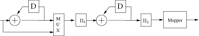
Figure 5.10: A specific manifestation of the generic transmitter schematic seen in Figure 5.4.
5.4.3 BER Performance
In our BER investigations, the RSC(2, 1, 2) code having the octal generator polynomials of (2/3) was invoked in Encoder/Decoder I. For the rate-1 Encoder II, again, the generator polynomial of 1/(1 + D) was used. Figure 5.10 shows a more specific manifestation of the generic transmitter schematic seen in Figure 5.4. The block length is L = 105bits. The activation order of the three SISO modules is [3 2 1 2 1 2] and this pattern is repeated 12 times.
Our BER results are depicted in Figure 5.11. In addition to the three-stage SISO system, the BER performance of the two-stage SISO system seen in Figure 5.1 and using a MMSE equalizer is also shown. Observe in Figure 5.11 that the two-stage SISO system performs better in the low-SNR region, while the three-stage SISO system has the edge in the medium to high SNR region, achieving an infinitesimally low BER for Eb/N0 values above 3 dB and hence closely matching the convergence threshold of Eb/N0 = 2.8dB predicted by the EXIT chart analysis of Figure 5.8. Although the two-stage scheme is of lower decoding complexity, it cannot outperform the AWGN BER bound, regardless of the number of iterations. To achieve a near-zero BER in the medium SNR range, the three-stage scheme has to be used. Additionally, as seen from Figure 5.11, the actual numbers of iterations required for achieving near-zero BER at Eb/N0 = 3dB, 3.5 dB, 4 dB and 5 dB are I = 12, 7, 5 and 4 respectively, which match the predictions of I = 10, 6, 5 and 3 seen in Table 5.2 quite well.
Figure 5.11: BER performance of the three-stage concatenation scheme of Figure 5.10 and the two-stage concatenation scheme of Figure 5.1 using a MMSE equalizer for transmission over the dispersive AWGN channel having a CIR of Equation (5.8). Note that for the three-stage concatenation scheme we used a specially selected activation order of the three SISO modules, namely one iteration is equivalent to an activation period of [3 2 1 2 1 2], where the numbers denote the indices of the SISO modules.

5.4.4 Decoding Trajectories
The mutual information vector of [IE(u3), IE(c2), IE(u2), IE(c1)] recorded during the simulations may be used to describe the evolution of the system status in the course of iterative decoding. They can be visualized in two 3D EXIT charts, resulting in the so-called decoding trajectories. More explicitly, Figure 5.12 shows the decoding trajectory associated with the evolution of IE(c1), IE(u3) and IE(c2). Similarly Figure 5.13 depicts the decoding trajectory associated with the evolution of IE(c1), IE(u3) and IE(u2). Note that each graph depicts one and only one extrinsic output of each SISO module. Hence, each time a SISO module is invoked, the decoding trajectory evolves in one dimension. For example, in Figure 5.12, the activation of the equalizer allows the trajectory to evolve along the IA(c2), IE(u3) axis, while the activation of Decoder II evolves the trajectory along the IE(c2), IA(u3) axis. Finally the activation of Decoder I triggers the evolution of the trajectory along the IA(u2), IE(c1) axis.
Figure 5.12: The decoding trajectories recorded at Decoder II’s output IE(c2), the equalizer’s output IE(u3) and Decoder I’s output IE(c1) for Eb/N0 = 4 dB. The EXIT function of the equalizer and that of Decoder II are also shown. Each time a SISO module is invoked, the decoding trajectory evolves in the dimension associated with the corresponding extrinsic information output.

Alternatively, the decoding process can also be visualized using two 2D graphs, namely one trajectory associated with the extrinsic outputs IE(u2) and IE(c1) of Figure 5.4, while the other is associated with the extrinsic outputs IE(u3) and IE(c2). These characterize the constituent decoder pairs of Decoder I and Decoder II, and of Decoder II and the equalizer of Figure 5.4, respectively. The former is depicted in Figure 5.14, which again characterizes the exchange of mutual information between Decoder I and the combined module of the equalizer and Decoder II. The vertical segments of the trajectory represent the activation of the combined equalizer and Decoder II module exchanging extrinsic information a certain number of times, while the horizontal segments represent a single activation of Decoder I.
For example, in the simulations we used an activation order of [3 2 1 2 1 2 ...]. At the beginning of the iterations the equalizer was activated, but given the architecture of Figure 5.4 and the activation regime assumed, neither the value of IE(u2) nor that of IA(c1) was changed; hence, the trajectory stayed at the point A0 in Figure 5.14. Then Decoder II was activated, resulting in an increased value of IE(u2), and hence the trajectory reached the point A1. Subsequently, Decoder I was activated, which increased the value of IE(c1), and hence the trajectory traversed to the point A2. Similarly, the segment between A2 and A3 represents the activation of Decoder II, the segment between A3 and A4 denotes the activation of Decoder I, and the segment between A4 and A5 corresponds to the activation of Decoder II. The segment between A5 and A6 represents the beginning of a new combined iteration cycle associated with similar decoding activations.
Figure 5.13: The decoding trajectories recorded at Decoder I’s output IE(c1), Decoder II’s output IE(u2) and the equalizer’s output IE(u3) for Eb/N0 = 4 dB. The EXIT function of Decoder II and that of Decoder I are also shown. Each time a SISO module is invoked, the decoding trajectory evolves in the dimension associated with the corresponding extrinsic information output.

Figure 5.15 shows the trajectory associated with the extrinsic outputs IE(u3) and IE(c2), which characterizes the exchange of mutual information between the equalizer and the combined module of Decoder II and Decoder I. The vertical segments of the trajectory represent a single activation of the equalizer, while the horizontal segments represent the activation of Decoder II and Decoder I at a certain number of times. Specifically, the activation schedule of [3 2 1 2 1 2 ...] is visualized as follows. After an initial activation of the equalizer, the trajectory traverses from B0 to B1. Then it remains at B1 after the activation of Decoder II and Decoder I. This is because the output IE(c2) of Decoder II remained zero after the first activation. However, these two activations are visualized in Figure 5.14 by the segment traversing from A0 to A1 while representing the activation of Decoder II. Similarly the segment spanning from A1 to A2 denotes the activation of Decoder I. Then the second activation of Decoder II triggers the evolution of the trajectory to the point B2 in Figure 5.15. The following activation of Decoder I does not change the trajectory in Figure 5.15, but is visualized by the segment spanning from A3 to A4 in Figure 5.14. Then the activation of Decoder II triggers a trajectory transition to B3. A new iteration cycle is indicated by the transition from B3 to B4. In conclusion, we surmise that the convergence behavior of a three-stage SISO system can be adequately visualized using two 2D EXIT charts.
Figure 5.14: The decoding trajectories measured at Decoder II’s output IE(u2) and Decoder I’s output IE(c1) for Eb/N0 = 4 dB. The activations of Decoder II cause the trajectory to grow along the y-dimension, while the activations of Decoder I cause the trajectory to grow along the x-dimension. The activation of the equalizer is not visualized. More explicitly, the trajectories can be interpreted as [EQ: A0, DEC2: A0 → A1, DEC1: A1 → A2, DEC2: A2 → A3, DEC1: A3 → A4, DEC2: A4 → A5], where EQ denotes the activation of the equalizer and DEC1/DEC2 represent the activations of Decoders I and II respectively.

5.4.5 Effects of Interleaver Block Length
As described in Section 4.2.2.3, EXIT functions are usually obtained by recording the extrinsic outputs of the SISO decoders, given certain a priori inputs. Since the a priori LLRs are artificially generated using the Gaussian model, they are independent of each other. However, this assumption is not entirely valid in real systems, where the a priori inputs are generated by the interleaved extrinsic outputs of the adjacent SISO decoders. The independence assumption only holds for sufficiently large interleaver block lengths and for the first few iterations. Hence it transpires that the analysis using EXIT functions becomes more and more inaccurate upon increasing the number of iterations, and further aggravated when decreasing the interleaver’s block size.
We evaluated the performance of the three-stage system described in Section 5.4.3 for block length L = 105, 104, 103 and 102 bits using simulations, and the resultant BER performances are listed in Table 5.3. Since the outer code has a rate of R = 1/2 and the intermediate code has a unity rate, the length of both of the interleavers seen in Figure 5.4 is 2L. According to the EXIT chart analysis in Section 5.4.2.2, the convergence threshold of the three-stage system is 2.8 dB. For a block length of L = 105 bits, the system achieves convergence at about 3 dB, while the convergence is achieved at around 3.5 dB for L = 104 bits, at 5 dB for L = 103 bits and at around 11 dB for L = 102 bits.
Figure 5.15: The decoding trajectories measured at the equalizer’s output IE(u3) and Decoder II’s output IE(c2) for Eb/N0 = 4 dB. The activations of the equalizer cause the trajectory to grow along the y-dimension, while the activations of Decoder II cause the trajectory to grow along the x-dimension. The activation of Decoder I is not visualized. More explicitly, the trajectories can be interpreted as [EQ: B0 → B1, DEC2: B1, DEC1: B1, DEC2: B1 → B2, DEC1: B2, DEC2: B2 → B3].
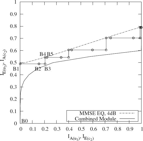
Table 5.3: BER performances for different block lengths after 12 iterations

Furthermore, for a given Eb/N0 value and fixed number of iterations, the BER increases upon decreasing the block length. For example, at Eb/N0 = 3dB, the BER increases from 2.0 × 10⁻⁶ to 1.6 × 10⁻¹ when the block length decreases from 105 to 102. This effect can also be visualized in the EXIT chart of Figure 5.16. For instance, the decoding trajectories of the systems using block lengths of L = 105, 104, 103 and 102 at Eb/N0 = 3dB are depicted in Figure 5.16. It can be seen that upon decreasing the block length the decoding trajectory drifts away from the EXIT curves more and more severely. In other words, the extrinsic information outputs of each SISO decoder become less than the EXIT chart predictions, resulting in increasing BERs.
Additionally, we show the achievable coding gain of the three-stage system at BER = 10−4 in Figure 5.17. Here, the coding gain is defined as the reduction of the required Eb/N0 when using the three-stage system as opposed to the uncoded system (i.e. when only MMSE equalization is employed without channel coding, using a block length of L = 105 bits). It can be seen that the maximum achievable coding gain decreases upon decreasing the block length. In comparison with the system employing the block length of L = 105 bits, the maximum coding gain of the system using a block length of L = 104 bits is decreased by less than 1 dB, while it is decreased by about 2 dB for the system using a block length of L = 103 bits and around 8 dB for L = 102 bits. Moreover, for L = 105 and L = 104, less than 0.5 dB iteration gain is achieved after I = 8 iterations, while for L = 103 the iteration gain diminishes after I = 6 iterations, and for L = 102 only a marginal iteration gain is obtained after I = 2 iterations.
5.5 Approaching the Channel Capacity Using EXIT-Chart Matching and IRCCs
In Section 5.4.2.2, we optimized the outer code of the three-stage system for achieving the lowest possible convergence threshold. The optimization was carried out by searching for different generator polynomials for the convolutional codes used. The lowest achievable convergence threshold was about 2.8 dB, when using a RSC(2, 1, 2) code having octally represented generator polynomials of 2/3. In this section we will investigate whether we can reduce this threshold further down by considering the area properties of EXIT charts.
5.5.1 Area Properties of EXIT Charts
Let us now discuss the relevance of the EXIT chart area ![]() I beneath the inverted outer EXIT function and
I beneath the inverted outer EXIT function and ![]() I beneath the inner EXIT function. Various proofs relating to these areas were provided in [204, 267] for the case when the a priori LLRs are provided for the respective APP SISO decoder over a Binary Erasure Channel (BEC) having either zero magnitudes or infinite magnitudes (and the correct sign). However, it has been shown that the shapes of the EXIT functions do not significantly depend on the particular channel considered [268], and hence the results discussed in this section hold approximately for more general channels.
I beneath the inner EXIT function. Various proofs relating to these areas were provided in [204, 267] for the case when the a priori LLRs are provided for the respective APP SISO decoder over a Binary Erasure Channel (BEC) having either zero magnitudes or infinite magnitudes (and the correct sign). However, it has been shown that the shapes of the EXIT functions do not significantly depend on the particular channel considered [268], and hence the results discussed in this section hold approximately for more general channels.
In [204, 267], the area ![]() I beneath the inverted EXIT function of an optimal outer APP SISO decoder having a coding rate of RI was shown to be given by
I beneath the inverted EXIT function of an optimal outer APP SISO decoder having a coding rate of RI was shown to be given by
Figure 5.16: Decoding trajectories of the system of Figure 5.4 using different block lengths at Eb/N0 = 3 dB.

In the case where this outer code is serially concatenated with a RII-rate inner code that is employed for protecting Mmod-ary modulated transmissions, the effective throughput η in bits of source information per channel use is given by
As described in Section 4.3, maintaining an open EXIT chart tunnel is a necessary condition for achieving iterative decoding convergence to an infinitesimally low probability
Figure 5.17: Achievable coding gain of the three-stage system of Figure 5.4 at BER = 10–4, when employing various block lengths and different numbers of iterations.

of Iterations of error. Since an open EXIT chart tunnel can only be created if the EXIT chart area beneath the inverted outer EXIT function ![]() I is less than that beneath the inner code’s EXIT function
I is less than that beneath the inner code’s EXIT function ![]() II, we have
II, we have ![]() I <
I < ![]() II and hence maintaining
II and hence maintaining
constitutes a necessary condition for the support of iterative decoding convergence to an infinitesimally low probability of error.
In the case where we have RII = 1 and an optimal inner APP SISO decoder is employed, [204, 267] showed that
where C is the Discrete-Input Continuous-Output Memoryless Channel’s (DCMC’s) capacity [269] expressed in bits of source information per channel use. Hence, in the case where RII = 1 and an optimal inner APP SISO decoder is employed,
constitutes a necessary condition for the support of iterative decoding convergence to an infinitesimally low probability of error. Note that this is as Shannon stated in his seminal publication of 1948 [133].
However, in the case where we have RII < 1 or a suboptimal inner APP SISO decoder is employed, [204, 267] showed that
where ![]() is the attainable DCMC capacity. More explicitly, in this case some capacity loss occurs, since the necessary condition for iterative decoding convergence to an infinitesimally low probability of error to be supported becomes
is the attainable DCMC capacity. More explicitly, in this case some capacity loss occurs, since the necessary condition for iterative decoding convergence to an infinitesimally low probability of error to be supported becomes
Note that the EXIT chart area within an open EXIT chart tunnel ![]() II −
II − ![]() I is proportional to the discrepancy between the effective throughput and the (attainable) DCMC capacity. Hence, we may conclude that near-capacity transmissions are facilitated when a narrow, marginally open EXIT chart tunnel can be created for facilitating convergence to an infinitesimally low probability of error. This motivates the employment of irregular coding for EXIT chart matching, as will be discussed in the following sections.
I is proportional to the discrepancy between the effective throughput and the (attainable) DCMC capacity. Hence, we may conclude that near-capacity transmissions are facilitated when a narrow, marginally open EXIT chart tunnel can be created for facilitating convergence to an infinitesimally low probability of error. This motivates the employment of irregular coding for EXIT chart matching, as will be discussed in the following sections.
5.5.2 Analysis of the Three-Stage System
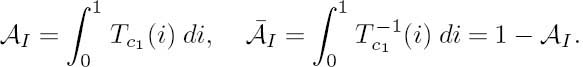
For convenience, we first redraw some of the previously used EXIT functions in Figure 5.18. According to the above-described area properties [116] of EXIT charts, the area under the EXIT curve of the inner code is approximately proportional to the channel capacity attained. Furthermore, the area under the inverted EXIT curve of the outer code is approximately equal to RI , where RI is the outer code’s rate. More explicitly, let ![]() I and
I and ![]() I be the areas under the outer code’s EXIT curve Tc1(i) and its inverse Tc1−1 (i), i ∈ [0, 1] respectively, which are expressed as
I be the areas under the outer code’s EXIT curve Tc1(i) and its inverse Tc1−1 (i), i ∈ [0, 1] respectively, which are expressed as
Similarly, we define the areas ![]() II and
II and ![]() II for the EXIT curve T′u2(i) of the combined module of the equalizer and Decoder II, as well as
II for the EXIT curve T′u2(i) of the combined module of the equalizer and Decoder II, as well as ![]() III and
III and ![]() III for the EXIT curve Tu3(i) of the inner equalizer. Then we have
III for the EXIT curve Tu3(i) of the inner equalizer. Then we have
and for BPSK modulation and MAP equalization
where CUI is the uniform-input capacity of the communication channel seen in the schematic of Figure 5.4.
Specifically, in Figure 5.18 the area under the EXIT curve of the MAP equalizer is ![]() III ≈ 0.59 and the area under the EXIT curve of the MMSE equalizer is
III ≈ 0.59 and the area under the EXIT curve of the MMSE equalizer is ![]() ′III ≈ 0.57. When expressed in terms of bits per channel use, these values approximate the channel’s capacity. The slight throughput loss of the latter is due to the employment of the MMSE criterion, which is inferior to the MAP criterion. Since the intermediate code has a unity rate, the area
′III ≈ 0.57. When expressed in terms of bits per channel use, these values approximate the channel’s capacity. The slight throughput loss of the latter is due to the employment of the MMSE criterion, which is inferior to the MAP criterion. Since the intermediate code has a unity rate, the area ![]() II under the EXIT curve of the combined module is equal to
II under the EXIT curve of the combined module is equal to ![]() ′III. In order to achieve convergence, there has to be an open tunnel between the EXIT curve of the combined module and that of the outer code. Accordingly we have
′III. In order to achieve convergence, there has to be an open tunnel between the EXIT curve of the combined module and that of the outer code. Accordingly we have ![]() ′III >
′III > ![]() I or
I or ![]() II >
II > ![]() I. Hence the area under the EXIT curve of the MMSE equalizer is equal to the maximum achievable information rate when using MMSE equalization, which is achieved when the EXIT curve of the outer code is perfectly fitted to the EXIT curve of the combined module. According to these area properties, the channel capacity derived for a uniformly distributed input and the maximum information rate achieved when using MAP/MMSE equalization may be readily obtained for the three-path channel of Equation (5.8), which is depicted as a function of Es/N0 in Figure 5.19. It can be seen that, compared with MAP equalization, there is an inherent information rate loss when employing the MMSE equalization, especially at high channel SNRs. The achievable information rates of the systems employing rate-1 intermediate codes are also plotted, and these show negligible information rate loss.
I. Hence the area under the EXIT curve of the MMSE equalizer is equal to the maximum achievable information rate when using MMSE equalization, which is achieved when the EXIT curve of the outer code is perfectly fitted to the EXIT curve of the combined module. According to these area properties, the channel capacity derived for a uniformly distributed input and the maximum information rate achieved when using MAP/MMSE equalization may be readily obtained for the three-path channel of Equation (5.8), which is depicted as a function of Es/N0 in Figure 5.19. It can be seen that, compared with MAP equalization, there is an inherent information rate loss when employing the MMSE equalization, especially at high channel SNRs. The achievable information rates of the systems employing rate-1 intermediate codes are also plotted, and these show negligible information rate loss.
Figure 5.18: EXIT functions of the MMSE equalizer, the MAP equalizer and the combined module of the MMSE equalizer and Decoder II at Eb/N0 = 2.8 dB, as well as the EXIT function of the outer RSC(2, 1, 2) code.

Figure 5.19: The achievable information rate for systems employing MAP/MMSE equalization for transmission over the three-path channel of Equation (5.8).

As seen from Figure 5.18, there is an open tunnel between the EXIT curve of the combined module and that of the outer RSC code at the convergence threshold of Eb/N0 = 2.8 dB; i.e., we have ![]() II −
II − ![]() I > 0, which implies that the channel capacity is not reached. On the other hand, if we fix the system’s throughput to 0.5 bits per channel use, the convergence threshold may be further lowered, provided that a matching outer code can be found. More explicitly, we found that the area under the EXIT curve of the equalizer at Eb/N0 = 1.6 dB (or equivalently at Es/N0 = −1.4 dB) is about 0.50. Hence our task now is to search for an outer code whose EXIT curve is perfectly matched to that of the combined module of the equalizer and Decoder II, so that the maximum information rate is achieved.
I > 0, which implies that the channel capacity is not reached. On the other hand, if we fix the system’s throughput to 0.5 bits per channel use, the convergence threshold may be further lowered, provided that a matching outer code can be found. More explicitly, we found that the area under the EXIT curve of the equalizer at Eb/N0 = 1.6 dB (or equivalently at Es/N0 = −1.4 dB) is about 0.50. Hence our task now is to search for an outer code whose EXIT curve is perfectly matched to that of the combined module of the equalizer and Decoder II, so that the maximum information rate is achieved.
Irregular codes, such as irregular LDPC codes, irregular RA codes [270] and IRCCs [80, 81], are reported to have flexible EXIT characteristics, which can be optimized to match the EXIT curve of the combined equalizer and Decoder II module, in order to create an appropriately shaped EXIT-chart convergence tunnel. For the sake of simplicity, IRCCs are considered in the forthcoming section.
5.5.3 Design of Irregular Convolutional Codes
The family of IRCCs was proposed in [80, 81]. It consists of a set of convolutional codes having different code rates. They were specifically designed with the aid of EXIT charts [98], for the sake of improving the convergence behavior of iteratively decoded systems. To be more specific, an IRCC is constructed from a family of P subcodes. First, a rate-r convolutional parent code C1 is selected and the (P − 1) remaining subcodes Ck of rate rk > r are obtained by puncturing. Let L denote the total number of encoded bits generated from the K uncoded information bits. Each subcode encodes a fraction αkrkL of the original uncoded information bits and generates αkL encoded bits. Given our overall average code rate target of R ∈ [0, 1], the weighting coefficient αk has to satisfy

Clearly, the individual code rates rk and the weighting coefficients αk play a crucial role in shaping the EXIT function of the resultant IRCC. For example, in [81] a family of P = 17 subcodes were constructed from a systematic, rate-1/2, memory-4 parent code defined by the generator polynomial (1, g1/g0), where g0 = 1 + D + D4 is the feedback polynomial and g1 = 1 + D2 + D3 + D4 is the feed-forward one. Higher code rates may be obtained by puncturing, while lower rates are created by adding more generators and by puncturing under the constraint of maximizing the achievable free distance. The two additional generators used are g2 = 1 + D + D2 + D4 and g3 = 1 + D + D3 + D4. The resultant 17 subcodes of [81] have coding rates spanning from 0.1, 0.15, 0.2, ... to 0.9.
Figure 5.20: EXIT functions of the 17 subcodes in [81].

The IRCC constructed using this procedure has the advantage that the decoding of all subcodes may be performed using the same parent code trellis, except that at the beginning of each block of αkrkL number of trellis transitions/sections corresponding to the subcode Ck the puncturing pattern has to be restarted. Trellis termination is necessary only after all of the K uncoded information bits have been encoded.
The EXIT function of an IRCC can be obtained from those of its subcodes. Denote the EXIT function of the subcode k as Tc1, k(IA(c1)). Assuming that the trellis segments of the subcodes do not significantly interfere with each other, which might change the associated transfer characteristics, the EXIT function Tc1(IA(c1)) of the target IRCC is the weighted superposition of the EXIT function Tc1, k(IA(c1)) [81], yielding

For example, the EXIT functions of the 17 subcodes used in [81] are shown in Figure 5.20. We now optimize the weighting coefficients, {αk}, so that the IRCC’s EXIT curve of Equation (5.29) matches the combined EXIT curve of Equation (5.17). The area under the combined EXIT curve of Equation (5.17) at Eb/N0 = 1.8 dB is ![]() II ≈ 0.51, which indicates that this Eb/N0 value is close to the lowest possible convergence threshold for a system having an outer coding rate of RI = 0.5. We optimize T(IA(c1)) of Equation (5.29) at Eb/N0 = 1.8 dB by minimizing the square of the error function
II ≈ 0.51, which indicates that this Eb/N0 value is close to the lowest possible convergence threshold for a system having an outer coding rate of RI = 0.5. We optimize T(IA(c1)) of Equation (5.29) at Eb/N0 = 1.8 dB by minimizing the square of the error function
subject to the constraints of (5.28) and e(i) >0 over all i:

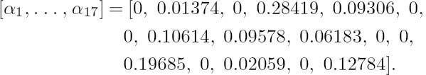
In more tangible physical terms, we minimize the area between the projected EXIT curve and the EXIT curve of the outer code, as seen in Figure 5.8. This results in a good match between the two curves, ultimately leading to a narrow EXIT-chart tunnel, which implies a near-capacity operation attained at the cost of a potentially high number of decoding iterations. The associated high complexity is characteristic of schemes operating beyond the Shannonian cut-off rate. The curve-fitting problem portrayed in Equation (5.31) is a quadratic programming problem, which can be solved by the gradient-descent-based iterative solution proposed in [80]. With the aid of this algorithm [80], the optimized weighting coefficients are obtained as
The resultant EXIT curve of the optimized IRCC is shown in Figure 5.21.
Note that the ability of EXIT chart matching to create narrow but still open EXIT chart tunnels depends on the availability of a suite of component codes having a wide variety of EXIT function shapes. However, in general it is challenging to design component codes having arbitrary EXIT function shapes, motivating the irregular code design process depicted in Figure 5.22. This advocates the design of diverse candidate component codes, the characterization of their EXIT functions and the selection of a specific suite having a wide variety of EXIT function shapes, potentially involving a significant amount of ‘trialand-error’-based human interaction. Following this, EXIT chart matching may be achieved by selecting the component fractions, as described above. Throughout Part II of this book we shall describe a number of modifications to this process.
5.5.4 Simulation Results
Monte Carlo simulations were performed for characterizing both the IRCC design and the convergence predictions of Section 5.5.3. As our benchmark scheme, the RSC(2, 1, 2) code having octal generator polynomials of 2/3 was employed as Encoder I in the schematic of Figure 5.4. As our proposed scheme, the IRCC designed in Section 5.5.3 was used as Encoder I. The rest of the system components were the same for both schemes, and all of the system parameters are listed in Table 5.4.
Figure 5.23 depicts the BER performance of both schemes. It can be seen that after 12 iterations, the three-stage scheme employing an IRCC achieves a BER lower than 10−5 at about Eb/N0 = 2.4 dB, which outperforms the three-stage scheme using a regular RSC code by about 0.5 dB. Moreover, if more iterations are invoked, for example I = 30 iterations, the three-stage scheme employing an IRCC is capable of achieving convergence at Eb/N0 = 2 dB, which is very close to the convergence threshold of Eb/N0 = 1.8 dB predicted by the EXIT chart analysis. Hence, a total additional gain of about 1 dB is achievable by using the optimized IRCC.
Figure 5.21: The combined EXIT function of Equation (5.17) and the EXIT function of the optimized IRCC at Eb/N0 = 1.8 dB.

Figure 5.22: Conventional irregular coding design process.

Table 5.4: System parameters used in the simulations of Section 5.5.4
| Encoder I | Half-rate RSC(2, 1, 2) code, G = 2/3 or Half-rate IRCC of Equation (5.32) |
| Encoder II | Generator polynomials 1/3 |
| Modulation | BPSK |
| CIR | [0.407 0.815 0.407]T |
| Block length | L = 100 000 bits |
| Overall coding rate | 0.5 |
Figure 5.23: BER performances for the three-stage serial concatenation scheme of Figure 5.4 using both regular RSC code and IRCC for transmission over the dispersive AWGN channel having a CIR of Equation (5.8). The system parameters are outlined in Table 5.4.
The decoding trajectory recorded during our Monte Carlo simulations using the optimized IRCC is depicted in Figure 5.24. It can be seen that at Eb/N0 = 2 dB a narrow tunnel exists between the EXIT curve of the outer IRCC code and that of the combined module of the equalizer and Decoder II. Observe furthermore that the simulation-based recorded trajectory matches these EXIT curves quite closely, except for a few iterations close to the point of convergence. Furthermore, since the tunnel between the two EXIT curves is narrow, numerous iterations are required in order to enable the iterative receiver to converge to the point of (1, 1). When aiming to approach the channel capacity even more closely, the tunnel becomes even narrower, and therefore more iterations would be needed, resulting in a drastically increased complexity. At the same time, even longer interleavers will be required in order to ensure that the soft information exchanged between the SISO modules remains uncorrelated, so that the recorded decoding trajectory follows the EXIT curves. This is another manifestation of Shannon’s channel capacity theorem [1].
5.6 Rate Optimization of Serially Concatenated Codes
In Section 5.4.2 we have shown that by using a unity-rate intermediate code and a half-rate RSC(2, 1, 2) outer code, the three-stage system of Figure 5.4 became capable of achieving convergence at Eb/N0 = 2.8 dB, which is 1.4 dB away from the channel capacity achievable in case of uniformly distributed inputs, and 1.2 dB away from the maximum achievable information rate of MMSE equalization. Below we investigate the performance of the three-stage system, when employing an intermediate code having a rate of RII < 1. In other words, we fix the overall coding rate Rtot = 0.5 (i.e., we fix the system throughput to be 0.5 bits per channel use assuming BPSK), and optimize the rate allocation between the intermediate code and the outer code as well as their generator polynomials and puncturing matrix, so that convergence is achieved at the lowest possible Eb/N0 value.
Figure 5.24: The decoding trajectory of the three-stage system using IRCC at Eb/N0 = 2dB. The EXIT function of the IRCC, IE(c1) = Tc1(IA(c1)), and that of the combined module of the equalizer and Decoder II, IE(u2) = T′u2(IA(u2)), are also shown.

For simplicity, we limit our search space to regular convolutional codes having constraint lengths of K < 4. For the rate allocation between the intermediate code and the outer code, we consider two cases: R1II = 3/4, R1I = 2/3, and R2II = 2/3, R2I = 3/4. The rate-2/3 and rate-3/4 codes are generated by puncturing the rate-1/2 parent code, and the puncturing matrices used are listed in Table 5.5. An exhaustive search was carried out, and the combinations that exhibit good convergence properties are listed in Table 5.6. Furthermore, we depict the EXIT functions of the SCCs in Figure 5.25. Note that the EXIT function of each SCC was obtained by using the EXIT module of each component code, rather than by simulations. This incurs a substantially lower complexity.
Table 5.5: Puncturing matrices for generating rate-2/3 and rate-3/4 codes from rate-1/2 parent codes

Table 5.6: Optimized serially concatenated codes and the convergence thresholds of the corresponding three-stage systems

It can be seen from Table 5.6 that the lowest achievable convergence threshold of 2.2 dB is achievable by the SCC-A1/A2 and SCC-B4 schemes. This value is 0.6 dB lower than that of the system using rate-1 intermediate codes as discussed in Section 5.4. In order to verify our EXIT chart analysis, Monte Carlo simulations were also conducted, and the BER performance of the corresponding three-stage system using, for instance, the SCC-A2 scheme, is depicted in Figure 5.26. It can be seen that a BER of 10−5 is achieved at around Eb/N0 = 2.4 dB, which is close to our EXIT-chart prediction.
Although the three-stage system using an intermediate code having rate less than unity may achieve a lower convergence threshold than the system using a rate-1 intermediate code, as expected, the maximum achievable information rate is reduced. Let ![]() II be the area under the EXIT curve of the combined module of the inner equalizer and the intermediate decoder. According to the area properties of EXIT charts [116], the coding rate of the outer code RI
II be the area under the EXIT curve of the combined module of the inner equalizer and the intermediate decoder. According to the area properties of EXIT charts [116], the coding rate of the outer code RI
Figure 5.25: The EXIT functions of some of the optimized SCCs listed in Table 5.6.

should satisfy RI < ![]() II so that convergence may be achieved. Therefore the total coding rate Rtot
II so that convergence may be achieved. Therefore the total coding rate Rtot ![]() RIRII should satisfy Rtot < RIIAII. Since
RIRII should satisfy Rtot < RIIAII. Since ![]() II ≤ 1, it is evident that the system’s throughput is bounded by RII. For example, the achievable information rates of the systems using intermediate codes of rates of RII = {1, 3/4, 2/3} are depicted in Figure 5.27. It can also be seen that the maximum achievable information rate is affected by the constraint length of the intermediate code. Additional information rate loss is incurred by using a relatively low constraint length code.
II ≤ 1, it is evident that the system’s throughput is bounded by RII. For example, the achievable information rates of the systems using intermediate codes of rates of RII = {1, 3/4, 2/3} are depicted in Figure 5.27. It can also be seen that the maximum achievable information rate is affected by the constraint length of the intermediate code. Additional information rate loss is incurred by using a relatively low constraint length code.
Figure 5.26: BER performance of the three-stage system of Figure 5.4 when employing the SCC of SCC-A2 listed in Table 5.6 for transmission over the dispersive AWGN channel having a CIR of Equation (5.8). The block length of the input data is L = 105 bits.

Figure 5.27: Achievable information rates for systems employing MAP/MMSE equalization and various intermediate codes for transmission over the three-path channel of Equation (5.8).

5.7 Joint Source-Channel Turbo Equalization Revisited
In Section 4.4.4 we introduced a three-stage joint source and channel decoding as well as turbo equalization scheme, as depicted in Figures 4.40 and 4.41. Moreover, it was shown in Figure 4.42 that the iteratively detected amalgamated scheme significantly outperformed the separate source and channel decoding as well as the turbo equalization scheme. In our forthcoming discourse, we investigate the convergence behavior of the iterative-detectionaided amalgamated source–channel decoding and turbo equalization scheme with the aid of the EXIT-module-based convergence analysis technique described in Section 5.4.
Figure 5.28: The receiver schematic of the joint source–channel turbo equalization scheme described in Section 4.4.4.
For the sake of convenience, we redraw the iterative receiver structure in Figure 5.28, which is similar to the three-stage turbo-equalization-aided receiver of Figure 5.4. However, the channel equalizer considered here employs the APP equalization algorithm described in Section 4.4 instead of the MMSE equalization algorithm of Section 5.2. Furthermore, the intermediate decoder is constituted by a half-rate memory-4 RSC decoder and the outer decoder is constituted by the SISO VLC decoder characterized in Section 4.3. The rest of the system parameters are the same as in Table 4.2. As shown in Figure 5.28, the input of the iterative receiver is constituted by the ISI-contaminated channel observations, and after a number of joint channel equalization, channel decoding and source decoding iterations, which are performed according to a specific activation order, the source symbol estimates are generated.
Let us first consider the EXIT function of the combined module constituted by the channel equalizer and the channel decoder, which is shown in Figure 5.29 and indicated by a solid line with ‘+’ symbols. The EXIT function of the outer VLC decoder is also depicted using a solid line with ‘×’ symbols. It can be seen that at Eb/N0 = 1.5 dB an open tunnel is formed between the two EXIT functions, which implies that the amalgamated source–channel decoding and turbo equalization scheme is capable of converging to the point C2 of ![]() and hence an infinitesimally SER may be achieved. By contrast, if a separate source–channel decoding and turbo equalization scheme is employed, which implies that the VLC decoder is invoked once after a certain number of channel equalization and channel decoding iterations, the receiver can only converge to the relatively low mutual information point of C1, as indicated in Figure 5.29.
and hence an infinitesimally SER may be achieved. By contrast, if a separate source–channel decoding and turbo equalization scheme is employed, which implies that the VLC decoder is invoked once after a certain number of channel equalization and channel decoding iterations, the receiver can only converge to the relatively low mutual information point of C1, as indicated in Figure 5.29.
On the other hand, let us consider the EXIT function of the combined module constituted by the channel decoder and the VLC decoder, which is depicted in Figure 5.29 using a dense dashed line. The EXIT function of the outer channel equalizer is also shown, as a solid line. As expected, at Eb/N0 = 1.5 dB an open tunnel is formed between the two EXIT functions, and the receiver becomes capable of converging to the point C4 of ![]() which implies that residual errors may persist at the output of the channel equalizer, but, nonetheless, a near-zero probability of error can be achieved at the output of the channel decoder and the VLC decoder. By contrast, a conventional two-stage turbo equalization scheme consisting only of channel equalization and channel decoding without source decoding can only converge to the relatively low mutual information point of C3, as indicated in Figure 5.29.
which implies that residual errors may persist at the output of the channel equalizer, but, nonetheless, a near-zero probability of error can be achieved at the output of the channel decoder and the VLC decoder. By contrast, a conventional two-stage turbo equalization scheme consisting only of channel equalization and channel decoding without source decoding can only converge to the relatively low mutual information point of C3, as indicated in Figure 5.29.
Figure 5.29: EXIT chart of the joint source–channel turbo equalization receiver of Figure 5.28, where SSC-TE denotes the separate source–channel turbo equalization scheme, JSC-TE represents the joint source–channel turbo equalization scheme and TE represents the two-stage turbo equalization scheme.

In summary, when incorporating the outer VLC decoder into the iterative decoding process, the three-stage amalgamated source–channel turbo equalization scheme has a convergence threshold of about Eb/N0 = 1.5 dB, which is significantly lower than that of the separate source–channel turbo equalization scheme.
5.8 Summary and Conclusions
In this chapter we have investigated several three-stage serially concatenated turbo schemes from an EXIT-chart-aided perspective. As a result a number of system design guidelines were obtained, which are summarized below.
- The three-stage concatenation principle
The advocated system design principles are exemplified by an iterative three-stage MMSE equalization scheme, where the iterative receiver is constituted by three SISO modules, namely the inner MMSE equalizer, the intermediate channel decoder and the outer channel decoder. From the point of view of precoding, the inner equalizer and the intermediate decoder of Figure 5.4 may be regarded as a combined module and the EXIT function of this combined module is shown in Figure 5.7. Although the EXIT function of the stand-alone equalizer cannot reach the point of (1, 1) (i.e., Tc1(1) ≠ 1 c. f. Equation (5.12)), it can be seen that the EXIT function of the combined module can (i.e., T′u2(IA(u2) = 1, Eb/N0) = 1, c.f. Equation (5.17)). Therefore the three-stage system becomes capable of achieving the convergence point of (1, 1), which corresponds to an infinitesimally low BER. - Alternatively, the intermediate decoder and the outer decoder can be viewed as a combined module, which results in a serially concatenated turbo-like code. The EXIT function of this combined module is depicted in Figure 5.9. It can be seen that the combined module has steep EXIT characteristics. For example, after I = 10iterations between the intermediate decoder and the outer decoder, the EXIT function of the combined module reaches the upper bound value of 1 for any a priori information input larger than 0.6; i.e., we have T′c2(IA(c2)) = 1, ∀IA(c2) > 0.6. This characteristic matches that of the inner equalizer quite well and the corresponding three-stage system is capable of achieving IE(c2) = 1, which implies that we have IE(c1) = IA(u2) = 1 according to the EXIT characteristics of Decoder II, as seen in Figure 5.6a. Again, an infinitesimally low BER can be achieved.
- EXIT-chart matching-based optimization and the use of irregular codes
In the context of three-stage concatenations, the outer code is optimized, so that its EXIT function is matched to that of the combined module of the inner equalizer and the intermediate decoder, yielding the lowest Eb/N0 convergence threshold. Interestingly, we found in the context of Figure 5.8 that, as far as conventional convolutional codes are concerned, relatively weak codes having a short memory may result in the lowest convergence thresholds in the investigated three-stage context. This is due to the low initial value (IE(u2) = T′u2 (0, Eb/N0)) of the EXIT function of the combined module, which results in an undesirable EXIT function intersection with that of a strong code earlier than a weak code, as seen in Figure 5.18. Furthermore, if a well-designed IRCC is invoked as the outer code, the convergence threshold of the three-stage system may become even lower. For example, in our system of Section 5.5 employing an IRCC, a near-zero BER is achieved at Eb/N0 = 2dB, which is only about 0.3 dB away from the lowest achievable convergence threshold constituted by the capacity. - Rate optimization of SCCs
In addition to rate-1 codes, lower-rate intermediate codes may also be used in three-stage systems. Such systems have been shown in Figures 5.25 and 5.26 to exhibit lower convergence thresholds and better BER performances than those using rate1 intermediate codes and regular outer codes. Even lower convergence thresholds can be achieved if irregular outer codes are used; however, the decoding complexity typically becomes significantly higher. The disadvantage of using intermediate codes having RII < 1is the reduction of the maximum achievable information rate as seen in Figure 5.27; however, several SCCs having different intermediate coding rates can be designed and activated in order to render the channel coding scheme adaptive to the time-variant channel conditions. - Optimization of activation orders For multiple concatenation of more than two SISO modules, the activation order of the component decoders is an important issue, which may affect the computational complexity, delay and performance. With the aid of 1D and 2D EXIT functions, we are able to predict the number of three-stage activations required in order to achieve converge. It was observed in Table 5.2 that the component module that has the strongest error correction capability, for example the outer code, should be invoked more frequently, in order that the total number of three-stage activations is minimized. Moreover, considering the computational complexities of the component modules, their activation order should be tuned to achieve the target trade-off between fast convergence and low complexity. The activation order thus obtained is rather heuristic and might not be the optimal one. However, the optimal activation order would vary as a function of the channel SNR, the interleaver block length, the affordable total complexity etc. Hence, we surmise that the proposed heuristic techniques are adequate.
Additionally, like those of two-stage systems, the decoding/detection processes of the three-stage systems may be visualized using EXIT charts as decoding trajectories. We have shown in Section 5.4.4 that either two 3D EXIT charts or two 2D EXIT charts can be used to characterize the decoding process in terms of the associated mutual information exchange. Since 2D charts are easier to manipulate and interpret, they are preferable.
Finally, the analysis and design procedure advocated here may be applied in the context of diverse iterative receivers employing multiple SISO modules, such as the jointly designed source coding and space–time coded modulation schemes of [271, 272]. The MMSE equalizer used in the three-stage system of Figure 5.4 discussed here may also be replaced by an M-ary demapper or a MIMO detector, and the resultant system can be optimized with the aid of the methods proposed here. The design of further near-capacity systems constitutes our future research.
1Parts of this chapter are based on the collaborative research outlined in [211] © IEEE (2006), [213] © IEEE © IEEE (2009).