
Chapter 3
Sources and Source Codes
3.1 Introduction
This chapter, and indeed the rest of the book, relies on familiarity with the basic concepts outlined in Chapter 2, where a rudimentary introduction to VLCs, such as entropy codes and Huffman codes, and their benefits, was provided. This chapter primarily investigates the design of VLCs constructed for compressing discrete sources, as well as the choice of soft decoding methods for VLCs. First, in Section 3.2 appropriate source models are introduced for representing both discrete memoryless sources and discrete sources having memory. In order to map discrete source symbols to binary digits, source coding is invoked. This may employ various source codes, such as Huffman codes [9] and RVLCs [12] as well as VLEC codes [30]. Unlike channel codes such as convolutional codes, VLCs constitute nonlinear codes; hence the superposition of legitimate codewords does not necessarily yield a legitimate codeword. The design methods of VLCs are generally heuristic. As with channel codes, the coding rate of VLCs is also an important design criterion in the context of source codes, although some redundancy may be intentionally imposed in order to generate reversible VLCs, where decoding may be commenced from both ends of the codeword, or to incorporate error-correction capability. A novel code construction algorithm is proposed in Section 3.3, which typically constructs more efficient source codes in comparison with the state-of-the-art methods found in the literature.
The soft decoding of VLCs is presented in Section 3.4. In contrast with traditional hard decoding methods, processing binary ones and zeros, the family of soft decoding methods is capable of processing soft input bits, i.e. hard bits associated with reliability information, which are optimal in the sense of maximizing the a posteriori probability. Finally, the performance of soft decoding methods is quantified in Section 3.4.3, when communicating over AWGN channels.
3.2 Source Models
Practical information sources can be broadly classified into the families of analog and digital sources. The output of an analog source is a continuous function of time. With the aid of sampling and quantization an analog source signal can be transformed into its digital representation.
The output of a digital source is constituted by a finite set of ordered, discrete symbols, often referred to as an alphabet. Digital sources are usually described by a range of characteristics, such as the source alphabet, the symbol rate, the individual symbol probabilities and the probabilistic interdependence of symbols.
At the current state of the art, most communication systems are digital, which has a host of advantages, such as their ease of implementation using Very-Large-Scale Integration (VLSI) technology and their superior performance in hostile propagation environments. Digital transmissions invoke a whole range of diverse signal processing techniques, which would otherwise be impossible or difficult to implement in analog forms. In this monograph we mainly consider discrete-time, discrete-valued sources, such as the output of a quantizer.
3.2.1 Quantization
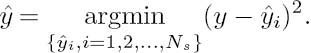
Source symbols with values having unequal probabilities of occurrence may be generated during the scalar quantization [164, 165] of real-valued source samples, for example. In scalar quantization, each real-valued source sample y is quantized separately. More specifically, an approximation ![]() of each source sample y is provided by one of Ns number of real-valued quantization levels {
of each source sample y is provided by one of Ns number of real-valued quantization levels {![]() i, i = 1, 2,..., Ns}. In each case, the selected quantization level
i, i = 1, 2,..., Ns}. In each case, the selected quantization level ![]() i is that particular one that has the smallest Euclidean distance from the source sample, according to
i is that particular one that has the smallest Euclidean distance from the source sample, according to
This selection is indicated using a source symbol having the corresponding value from the alphabet ![]() = {a1, a2,..., ai,..., aNs}. During inverse quantization, each reconstructed source sample
= {a1, a2,..., ai,..., aNs}. During inverse quantization, each reconstructed source sample ![]() approximates the corresponding source sample y using the quantization level
approximates the corresponding source sample y using the quantization level ![]() i that is indicated by the source symbol A. Owing to this approximation, quantization noise is imposed upon the reconstructed source samples. It may be reduced by employing a larger number of quantization levels Ns.
i that is indicated by the source symbol A. Owing to this approximation, quantization noise is imposed upon the reconstructed source samples. It may be reduced by employing a larger number of quantization levels Ns.
Furthermore, in Lloyd–Max quantization [164, 165] typically the K-means algorithm [233] is employed to select the quantization levels {![]() i, i = 1, 2,..., Ns} in order to minimize the imposed quantization noise that results for a given number of quantization levels Ns. This is illustrated in Figure 3.1 for the Ns =4-level Lloyd–Max quantization of Gaussian distributed source samples having a zero mean and unity variance. Observe that the Probability Density Function (PDF) of Figure 3.1 is divided into Ns = 4 sections by the decision boundaries, which are located halfway between each pair of adjacent quantization levels, namely
i, i = 1, 2,..., Ns} in order to minimize the imposed quantization noise that results for a given number of quantization levels Ns. This is illustrated in Figure 3.1 for the Ns =4-level Lloyd–Max quantization of Gaussian distributed source samples having a zero mean and unity variance. Observe that the Probability Density Function (PDF) of Figure 3.1 is divided into Ns = 4 sections by the decision boundaries, which are located halfway between each pair of adjacent quantization levels, namely ![]() i′ and
i′ and ![]() i′+1 for i′ = 1, 2,... Ns − 1. Here, each section of the PDF specifies the range of source sample values that are mapped to the quantization level
i′+1 for i′ = 1, 2,... Ns − 1. Here, each section of the PDF specifies the range of source sample values that are mapped to the quantization level ![]() i at its center of gravity, resulting in the minimum quantization noise.
i at its center of gravity, resulting in the minimum quantization noise.
The varying probabilities of occurrence {pi, i = 1, 2,..., Ns} of the Ns number of source symbol values generated during quantization may be determined by integrating the corresponding sections of the source sample PDF. Figure 3.1 shows the Ns =4 source symbol value probabilities of occurrence {pi, i = 1, 2,..., Ns} that result for the Ns = 4 level Lloyd–Max quantization of Gaussian distributed source samples.
Figure 3.1: Gaussian PDF for unity mean and variance. The x axis is labeled with the Ns = 4 Lloyd–Max quantization levels {![]() i, i = 1, 2,..., Ns} and Ns − 1 = 3 decision boundaries as provided in [164]. The decision boundaries are employed to decompose the Gaussian PDF into Ns = 4 sections. The integral pi of each PDF section is provided.
i, i = 1, 2,..., Ns} and Ns − 1 = 3 decision boundaries as provided in [164]. The decision boundaries are employed to decompose the Gaussian PDF into Ns = 4 sections. The integral pi of each PDF section is provided.

In the case where the source samples are correlated, Vector Quantization (VQ) [170] may be employed to generate source symbols with values having unequal probabilities of occurrence. In contrast with scalar quantization, where an individual source sample is mapped to each quantization level, VQ maps a number of correlated source samples to each so-called quantization tile. Quantization tiles that impose a minimum quantization noise may be designed using the Linde–Buzo–Gray (LBG) algorithm [170], which applies the K -means algorithm [233] in multiple dimensions.
3.2.2 Memoryless Sources
Following Shannon’s approach [1], let us consider a source A emitting one of Ns possible symbols from the alphabet ![]() = {a1, a2,..., ai,..., aNs} having symbol probabilities of {pi, i = 1, 2,..., Ns}. Here the probability of occurrence for any of the source symbols is assumed to be independent of previously emitted symbols; hence this type of source is referred to as a ‘memoryless’ source. The information carried by symbol ai is
= {a1, a2,..., ai,..., aNs} having symbol probabilities of {pi, i = 1, 2,..., Ns}. Here the probability of occurrence for any of the source symbols is assumed to be independent of previously emitted symbols; hence this type of source is referred to as a ‘memoryless’ source. The information carried by symbol ai is
The average information per symbol is referred to as the entropy of the source, which is given by

Figure 3.2: A two-state Markov model.

where H is bounded according to
and we have H = log2 Ns when the symbols are equiprobable.
Then the average source information rate can be defined as the product of the information carried by a source symbol, given by the entropy H, and the source emission rate Rs [symbols/second]:
3.2.3 Sources with Memory
Most analog source signals, such as speech and video, are inherently correlated, owing to various physical restrictions imposed on the analog sources [2]. Hence all practical analog sources possess some grade of memory, which constitutes a property that is also retained after sampling and quantization. An important feature of sources having memory is that they are predictable to a certain extent; hence, they can usually be more efficiently encoded than unpredictable memoryless sources can.
Predictable sources that exhibit memory can be conveniently modeled by Markov processes, as introduced in Section 2.6.1. A source having a memory of one symbol interval directly ‘remembers’ only the previously emitted source symbol, and, depending on this previous symbol, it emits one of its legitimate symbols with a certain probability, which depends explicitly on the state associated with this previous symbol. A one-symbol-memory model is often referred to as a first-order model.
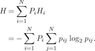
In general, Markov models are characterized by their state probabilities Pi = P(X = Xi), i = 1,..., N, where N is the number of states, as well as by the transition probability pij = P(Xj/Xi), where pij explicitly indicates the probability of traversing from state Xi to state Xj. At every state transition, they emit a source symbol. Figure 3.2 shows a two-state first-order Markov model as introduced in Figure 2.9, and repeated here for the reader’s convenience.
The entropy of a source having memory is defined as the weighted average of the entropies of the individual symbols emitted from each state, where weighting is carried out by taking into account the probability of occurrence of the individual states, namely Pi. In analytical terms, the symbol entropy for state Xi, i = 1,..., N is given by

The symbol entropies weighted by their probability of occurrence are summed, which effectively corresponds to averaging over all symbols, hence yielding the source entropy:
Finally, assuming a source symbol rate of Rs, the average information emission rate R of the source is given by
A widely used analytical Markov model is the Autoregressive (AR) model. A zero-mean random sequence y(n) is referred to as an AR process of order N if it is generated as follows:

where ε(k) is an uncorrelated zero-mean, random input sequence with variance σ2. Avariety of practical information sources are adequately modeled by the analytically tractable first-order Markov/AR model given by
where ρ is the correlation coefficient of the process y(k).
3.3 Source Codes
Source coding is the process by which each source symbol is mapped to a binary codeword; hence the output of an information source is converted to a sequence of binary digits. For a non-uniform Discrete Memoryless Source (DMS) the transmission of a highly probable symbol carries little information, and hence assigning the same number of bits to every symbol in the context of fixed-length encoding is inefficient. Therefore various variable-length coding methods are proposed. The general principle is that the source symbols that occur more frequently are assigned short codewords and those that occur infrequently are assigned long codewords, which generally results in a reduced average codeword length. Hence variable-length coding may also be viewed as a data compression method. Shannon’s source coding theorem suggests that by using a source encoder before transmission the efficiency of a system transmitting equiprobable source symbols can be arbitrarily approached [1].
Code efficiency can be defined as the ratio of the source information rate and the average output bit rate of the source encoder, which is usually referred to as coding rate in the channel coding community [8]. The most efficient VLCs are Huffman codes [9]. Besides code efficiency, there are other VLC design criteria that may be important in the application environment, such as having a high error resilience or a symmetric codeword construction. Thus both RVLCs [12, 20, 21] and VLEC codes [30] are proposed in the literature. We will describe these in the following sections.
Before proceeding further, we now provide some definitions.
3.3.1 Definitions and Notions
Let X be a code alphabet with cardinality1 q. In what follows, we shall assume that we have q = 2, although the results may readily be extended to the general case of q > 2. A finite sequence x = x1x2 ... xl of code symbols (or bits for binary alphabets) is referred to as a codeword over X of length l(x) = l, where each code symbol satisfies xi ![]() X, for all i = 1, 2,..., l. A set C of legitimate words is referred to as a code. Let the code C have Ns legitimate codewords c1, c2,..., cNs and let the length of cj be given by lj = l(cj), j = 1, 2,..., Ns. Without loss of generality, assume that we have l1 ≤ l2 ≤ ··· ≤ lNs. Furthermore, let K denote the number of different codeword lengths in the code C and let these lengths be given by L1, L2,..., LK, where we have L1 < L2 < ··· < LK, and the corresponding number of codewords having specific lengths is given by n1, n2,..., nK, where we have
X, for all i = 1, 2,..., l. A set C of legitimate words is referred to as a code. Let the code C have Ns legitimate codewords c1, c2,..., cNs and let the length of cj be given by lj = l(cj), j = 1, 2,..., Ns. Without loss of generality, assume that we have l1 ≤ l2 ≤ ··· ≤ lNs. Furthermore, let K denote the number of different codeword lengths in the code C and let these lengths be given by L1, L2,..., LK, where we have L1 < L2 < ··· < LK, and the corresponding number of codewords having specific lengths is given by n1, n2,..., nK, where we have ![]() Where applicable, we use the VLC
Where applicable, we use the VLC ![]() ={00, 11, 010, 101, 0110} as an example.
={00, 11, 010, 101, 0110} as an example.
Definition 1 The Hamming weight (or simply weight) of a codeword ci, w(ci), is the number of nonzero symbols in ci. The Hamming distance between two equal-length words, dh (ci, cj), is the number of positions in which ci and cj differ. For example, the Hamming distance between the codewords ‘00’ and ‘11’ is dh (00, 11) = 2, while dh (010, 101) = 3.
Definition 2 The minimum block distance dbk at the length of Lk for a VLC C is defined as the minimum Hamming distance between all codewords having the same length Lk, i.e. [29]
![]()
There are λ different minimum block distances, one for each different codeword length. However, if for some length Lk there is only one codeword, i.e. we have nk = 1, then in this case the minimum block distance for length Lk is undefined. For example, the minimum block distance at length two for the VLC ![]() = {00, 11, 010, 101, 0110} is db2, while db3=3 and db4 is undefined.
= {00, 11, 010, 101, 0110} is db2, while db3=3 and db4 is undefined.
Definition 3 The overall minimum block distance, bmin, of a VLC C is defined as the minimum value of dbk over all possible VLC codeword lengths k = 1, 2, ..., K, i.e. [29]
![]()
According to this definition, the overall minimum block distance of the VLC ![]() = {00, 11, 010, 101, 0110} is bmin = min(db2, db3) = 2.
= {00, 11, 010, 101, 0110} is bmin = min(db2, db3) = 2.
Definition 4 The Buttigieg–Farrell (B–F) divergence distance2 dd(ci, cj) between two different-length codewords ci = ci1 ci2 · · · cili and cj = cj1 cj2 · · · cjlj, where we have ci, cj ![]() C, li = l(ci) and lj = l(cj), is defined as the Hamming distance between the codeword sections spanning the common support of these two codewords when they are left-aligned; i.e., assuming lj < li) [29]:
C, li = l(ci) and lj = l(cj), is defined as the Hamming distance between the codeword sections spanning the common support of these two codewords when they are left-aligned; i.e., assuming lj < li) [29]:
![]()
For example, the B–F divergence distance between the codewords ‘00’ and ‘010’ is the Hamming distance between ‘00’ and ‘01,’ i.e. we have a common-support distance of dd (00, 010) = 1. Similarly, we have dd (00, 101) = 1, dd (00, 0110) = 1, dd (11, 010) = 1, dd (11, 101) = 1, dd (11, 0110) = 1, dd (010, 0110) = 1 and dd (101, 0110) = 2.
Definition 5 The minimum B–F divergence distance dmin of the VLC C is the minimum value of all the B–F divergence distances between all possible pairs of unequal length codewords of C, i.e. [29]
![]()
According to this definition, the minimum divergence distance of the VLC ![]() = {00, 11, 010, 101, 0110} is dmin = 1.
= {00, 11, 010, 101, 0110} is dmin = 1.
Definition 6 The B–F convergence distance dc (ci, cj) between two different-length codewords ci = ci1 ci2 · · · cili and cj = cj1 cj2 · · · cjlj, where we have ci, cj ![]() C, li = l(ci) and lj = l(cj), is defined as the Hamming distance between the codeword sections spanning the common support of these two codewords when they are right-aligned; i.e., assuming lj < li [29]:
C, li = l(ci) and lj = l(cj), is defined as the Hamming distance between the codeword sections spanning the common support of these two codewords when they are right-aligned; i.e., assuming lj < li [29]:
![]()
For example, the B–F convergence distance between the codewords ‘00’ and ‘010’ is the Hamming distance between ‘00’ and ‘10’, i.e. dc (00, 010) = 1. Similarly, we have dc (00, 101) = 1, dc (00, 0110) = 1, dc (11, 010) = 1, dc (11, 101) = 1, dc (11, 0110) = 1, dc (010, 0110) = 1 and dc (101, 0110) = 2.
Definition 7 The minimum B–F convergence distance cmin of the VLC C is the minimum value of all the B–F convergence distances between all possible pairs of unequal-length codewords of C, i.e. [29]
![]()
According to this definition, the minimum B–F divergence distance of the VLC ![]() = {00, 11, 010, 101, 0110} is cmin = 1.
= {00, 11, 010, 101, 0110} is cmin = 1.
Definition 8 The set of VLC codeword sequences consisting of a total number of N code symbols (or bits for binary codes) is defined as the extended code of order N of a VLC. Note that such codeword sequences may consist of an arbitrary number of VLC codewords. Let the set FN be the extended code of order N of the VLC C and the integer ηi be the number of VLC codewords that constitute an element of the set FN; then we have [29]
![]()
For example, F4 = {0000, 0011, 1100, 1111, 0110} is the extended code of order four for the VLC ![]() = {00, 11, 010, 101, 0110}.
= {00, 11, 010, 101, 0110}.
Definition 9 The free distance, df , of a VLC C is the minimum Hamming distance between any two equal-length VLC codeword sequences, which may consist of an arbitrary number of VLC codewords. With the aid of the definition of extended codes, the free distance of a VLC may be defined as the minimum Hamming distance in the set of all arbitrary extended codes, i.e. [29]
![]()
where Fn is the extended code of order n of C. It was found in [29, 30] that df is the most important parameter that determines the error-correcting capability of VLEC codes at high channel Signal-to-Noise Ratios (SNRs). The relationship between df, bmin, dmin and cmin is described by the following theorem.
Theorem 1 The free distance df of a VLC is lower bounded by [29]
![]()
For the proof of the theorem please refer to [29]. According to this theorem, the free distance of the VLC ![]() = {00, 11, 010, 101, 0110} is df = min(2,1 + 1) = 2.
= {00, 11, 010, 101, 0110} is df = min(2,1 + 1) = 2.
Definition 10 Let A be a memoryless data source having an alphabet of {a1, a2, ..., aNs}, where the elements have a probability of occurrence given by pi, i = 1, 2, ..., Ns. The source A is encoded using the code C by mapping symbol ai to codeword ci for all indices i = 1, 2, ..., Ns. Then the average codeword length ![]() is given by
is given by

where li = l(ci) represents the length of the codeword ci.
Definition 11 AVLC’s efficiency or coding rate, η, is defined as

where H (A) is the entropy of source A, while the VLC’s redundancy, , is defined as

3.3.2 Some Properties of Variable-Length Codes
Non-Singular Codes
A code C is said to be non-singular if all the codewords in the code are distinct. Both fixed and variable-length codes must satisfy this property in order to be useful.
Unique Decodability
A code C is said to be uniquely decodable if we can map a string of codewords uniquely and unambiguously back to the original source symbols. It is plausible that all fixed-length codes that are non-singular are also uniquely decodable. However, this is not true in general for variable-length codes.
A necessary and sufficient condition for the existence of a uniquely decodable code is provided by the McMillan inequality [234].
Theorem 2 A necessary and sufficient condition for the existence of a uniquely decodable code having codeword lengths of l1, l2, ..., ls is that we have [234]

where qis the cardinality of the code alphabet.
Instantaneous Decodability
For practical applications, it is required that the decoding delay should be as low as possible in order to facilitate real-time interactive communications. The minimum possible decoding delay is achieved when a codeword becomes immediately decodable as soon as it was completely received. Any delay lower than this would imply that the code is redundant. A code satisfying this property is referred to as an instantaneously decodable code [235]. It is plausible that for a code to satisfy this property none of its codewords may constitute a prefix of another codeword. Therefore, these codes are also known as prefix codes [235]. Hence, prefix codes are uniquely decodable and have a decoding delay of at most ls (maximum codeword length) bit duration.
Interestingly enough, McMillan’s inequality, given in [234], is also a necessary and sufficient condition for the existence of a prefix code having codeword lengths of l1, l2, ..., ls, which was stated as the Kraft inequality [236]. Chronologically, the proof of this inequality was provided in [236] before that of McMillan’s [234].
3.3.3 Huffman Code
Huffman codes were named after their inventor, D. A. Huffman [9], and because of their high coding efficiency they have been widely adopted in both still image and video coding standards [2]. Huffman codes are optimum in the sense that the average number of binary digits required to represent the source symbols is as low as possible, subject to the constraint that the codewords satisfy the above-mentioned prefix condition, which allows the received sequence to be uniquely and instantaneously decodable.
Table 3.1: An example of RVLCs

The construction of Huffman codes is fairly straightforward and is described in many textbooks [2, 235], and thus is omitted here. It is noteworthy nonetheless that there are more possible Huffman trees than just one for a given source; i.e., the Huffman code construction is not necessarily unique.
Amongst the diverse variants a meritorious one is the canonical Huffman code, which is defined as the code having the following characteristics [237]:
- Shorter codewords have a numerically higher value than longer codewords, provided that short codewords are filled with zeros to the right so that all codewords have the same length.
- For a specific codeword length, the corresponding numerical values increase monotonically upon the decrease of the source symbol probabilities.
For example, the code {11, 10, 01, 001, 000} is the canonical Huffman code for the source given in Table 3.1. It can be seen that we have (110)2 = (6)10 > (100)2 =(4)10 > (010)2 =(2)10 > (001)2 =(1)10 > (000)2 =(0)10, where 0 denotes the extra zeros that are appended to the short codewords. Hence the above-mentioned properties of canonical Huffman codes are satisfied. In general, the canonical Huffman code has the minimum total sum of codeword-lengths Σ li and simultaneously the minimum maximum codeword length Lmax in addition to the minimum average codeword-length ![]() , while allowing fast instantaneous decoding [33]. The construction of this code was described, for example, in [237].
, while allowing fast instantaneous decoding [33]. The construction of this code was described, for example, in [237].
3.3.4 Reversible Variable-Length Codes
Due to the variable-length nature of Huffman codes, they are very sensitive to errors that occur in noisy environments. Even a single-bit error is extremely likely to cause loss of synchronization, which is the term often used to describe the phenomenon of losing track of the beginning and end of VLCs, when a single error renders a VLC codeword unrecognizable, and hence the data received after the bit error position becomes useless until a unique synchronization word is found.
As a potential remedy, RVLCs [12–14, 20–24] have been developed for the sake of mitigating the effects of error propagation. As the terminology suggests, RVLCs often have a symmetric construction, i.e. they have the same bit-pattern both at their beginning and at their end; this facilitates instantaneous decoding in both forward and backward directions, so that we can recover the correct data with a high probability from the received data even when errors occur. To achieve this, a RVLC must satisfy both the so-called prefix and suffix conditions, which implies that no codeword is allowed to be a prefix or a suffix of any other codeword. Thus RVLCs are also known as ‘fix-free’ codes. The conditions for the existence of RVLCs and their properties were studied in [25–27].
Apart from the above-mentioned symmetric RVLC construction, asymmetric RVLCs also exist. For the same source, a symmetric RVLC generally has a higher average code length and thus becomes less efficient than an asymmetric RVLC. However, a symmetric RVLC has the benefit of requiring a single decoding table for bidirectional decoding, while an asymmetric RVLC employs two. Hence symmetric RVLCs might be preferable for memory-limited applications. Table 3.1 shows an example of both a symmetric and an asymmetric RVLC. In the following sections we discuss the construction of RVLCs for a given source.
3.3.4.1 Construction of RVLCs
The constructionof RVLCs was studied in [12, 20–24]. Most RVLC constructions commence from a Huffman code designed for the source concerned, and then replace the Huffman codewords by identical-length codewords that satisfy both the above-mentioned prefix and suffix conditions, as necessary. If the number of valid reversible codewords is insufficient, longer reversible codewords have to be generated and assigned, resulting in an increased redundancy. Hence a lower code efficiency is expected. Viewing this process of mapping RVLCs to Huffman codes from a different perspective, it is plausible that at a given codeword length we are likely to run out of legitimate RVLCs owing to their ‘fix-free’ constraint, typically requiring length extension. In contrast, if there are more RVLC candidate codewords than necessary, different codeword selection mechanisms may be applied. For example, the Maximum Symmetric-Suffix Length (MSSL) scheme [20] may be used for designing symmetric RVLCs, or the Minimum Repetition Gap (MRG) [21] metric and the so-called ‘affix index’ [23] metric may be invoked for designing asymmetric RVLCs.
The number of codewords of a certain length that satisfy both the prefix and the suffix condition depends on the previously assigned (shorter) RVLC codewords. This dependency was not considered in [12], which hence resulted in reduced-efficiency RVLCs. In [21] it was conjectured that the number of available codewords of any length depends on the above-mentioned MRG metric associated with the shorter RVLC codewords. The codeword assignment policy in [21] was base on MRG and typically produced more efficient codes than the algorithm advocated in [12]. In [23] the formal relationship between the number of available RVLC codewords of any length and the structure of shorter RVLC codewords was established. Based on this relationship, the authors proposed a new codeword selection mechanism, which rendered the ‘length-by-length’ approach optimal. However, the computational complexity imposed is generally quite high. More details of the MRG-based algorithm [21], which is denoted as Algorithm A.1, and the affix index-based algorithm [23] denoted as Algorithm A.2 can be found in Appendix A.
Both Algorithm A.1 [21] and Algorithm A.2 [23] attempt to match the codeword length distribution of the RVLC to that of the corresponding Huffman code. Since a RVLC has to satisfy the suffix condition in addition to the prefix condition, the desirable codeword length distribution of a Huffman code is usually not matched by that of the RVLC for the same source.
Moreover, both the value of the minimal average codeword length and the optimal codeword length distribution of the RVLC are unknown for a given source. If we find the necessary and sufficient condition for the existence of a RVLC, finding the optimal codeword length distribution would be a constrained minimization problem. More explicitly, given the source symbol probabilities, the problem is to find a codeword length distribution that minimizes the average codeword length, while satisfying the necessary and sufficient condition at the same time. Some results related to this existence condition have been reported in [25–27, 238]; however, even the existence of a general necessary and sufficient condition is uncertain. Therefore, later in this section we propose a heuristic method for finding an improved codeword length distribution.
The proposed algorithm bases its codeword selection procedure on that of the procedures proposed in [21] or [23] and attempts to optimize the codeword length distribution of the resultant RVLC length by length. The construction procedure3 is given as Algorithm 3.1.
| Algorithm 3.1 | |
|
Step 1: Employ Algorithm A.1 or Algorithm A.2 of Appendix A to construct an initial RVLC, and calculate the length vector, n, which records the numbers of codewords at different lengths, i.e. the histogram of the VLC codewords’ lengths. Step 2: Increase the number of required codewords at length l by one, and decrease the number of required codewords at the maximum codeword length Lmax by one, yielding n(l):= n(l) + 1, n(Lmax):= n(Lmax) − 1. Use Algorithm A.1 or Algorithm A.2 of Appendix A to construct an RVLC based on the modified length distribution. Step 3: Recalculate the average codeword length Step 4: Repeat Steps 2 and 3 until the last level is reached. |
|
3.3.4.2 An Example Construction of a RVLC
In the following, we will demonstrate the construction procedure of our Algorithm 3.1 by using an example. The specific source for which our RVLC example is designed is the English alphabet shown in Table 3.3.
The construction procedure is summarized in Table 3.2. At the first iteration, the length vector is initialized to that of the Huffman code, namely n =[0027751112], and Tasi’s algorithm [21] (Algorithm A.1) is invoked to construct an initial RVLC, resulting in a length distribution of n =[0027435212]and an average codeword length of ![]() =4.30675. Then our length-distribution optimization procedure commences. Firstly, the number of codewords n(3)required at the length of l = 3 is increased by one. For the sake of maintaining the total number of codewords, the number of codewords n(10)required at the length of l = 10 is decreased by one. Therefore the desired length distribution becomes n =[0037435211], as shown in the second row of Table 3.2. Then Algorithm A.1 is invoked again to construct a RVLC according to the new length distribution, and the resultant average codeword length becomes
=4.30675. Then our length-distribution optimization procedure commences. Firstly, the number of codewords n(3)required at the length of l = 3 is increased by one. For the sake of maintaining the total number of codewords, the number of codewords n(10)required at the length of l = 10 is decreased by one. Therefore the desired length distribution becomes n =[0037435211], as shown in the second row of Table 3.2. Then Algorithm A.1 is invoked again to construct a RVLC according to the new length distribution, and the resultant average codeword length becomes ![]() =4.25791. Since the average codeword length of the new RVLC is lower than that of the old one, the code construction procedure continues to increase the number of codewords required at the length of l = 3 during the third iteration. However, the resultant RVLC now has an increased average codeword length of
=4.25791. Since the average codeword length of the new RVLC is lower than that of the old one, the code construction procedure continues to increase the number of codewords required at the length of l = 3 during the third iteration. However, the resultant RVLC now has an increased average codeword length of ![]() =4.26231; hence the code construction procedure has to restore the length vector to that of the RVLC obtained at the end of the second iteration, which is n =[00365222231]. Then the code construction procedure attempts to increase the number of codewords required at the next level, i.e. at the length of l = 4. Hence the desired length distribution at the beginning of the fourth iteration becomes n =[00375222230]. This procedure is repeated until the last level has been reached. As a result, the best RVLC having the minimum average codeword length is found at the end of the 12th iteration.
=4.26231; hence the code construction procedure has to restore the length vector to that of the RVLC obtained at the end of the second iteration, which is n =[00365222231]. Then the code construction procedure attempts to increase the number of codewords required at the next level, i.e. at the length of l = 4. Hence the desired length distribution at the beginning of the fourth iteration becomes n =[00375222230]. This procedure is repeated until the last level has been reached. As a result, the best RVLC having the minimum average codeword length is found at the end of the 12th iteration.
Table 3.2: An example construction of a RVLC designed for the English alphabet

†The desired RVLC length distribution: the arrows pointing upwards imply that the values at those positions have been increased by one, while arrows pointing downwards imply the opposite.
‡The actual length distribution of the resultant RVLC after each iteration: the underlines indicate the numbers that will be changed in the next iteration.
§Decides the next step of the code generator, which depends on the resultant average codeword length.
3.3.4.3 Experimental Results
Table 3.3 compares the RVLCs designed for the English alphabet, constructed using the proposed algorithm (invoking Algorithm A.1 of Appendix A for the initial construction), and the algorithms published in [12, 21, 23]. As a benefit of its improved length distribution, Algorithm 3.1 yields a RVLC construction of the highest efficiency. For example, compared with the algorithms in [12] and [21], the average codeword length is reduced by 2.8% and 1.5% respectively.
Table 3.3: VLCs for the English alphabet

In [24] Lin et al. proposed two so-called backtracking-based construction algorithms for asymmetric RVLCs. In comparison with the algorithm of [21], one of the algorithms in [24] is capable of achieving a lower average codeword length at the cost of an equal or higher maximum codeword length, while the other algorithm of [24] is capable of reducing the maximum codeword length at the expense of an increased average codeword length. Table 3.4 compares the achievable performance of the algorithm proposed here with that of various benchmarks, based on the Canterbury Corpus file set (available at http://corpus.canterbury.ac.nz), which was designed specifically for testing new compression algorithms. It shows that our Algorithm 3.1 of Section 3.3.4.1 is capable of reducing both the average codeword length and the maximum codeword length at the same time.
In [22] Lakovic et al. proposed a construction algorithm based on the MRG metric for designing RVLCs having a free distance of df = 2, which significantly outperformed the regular RVLCs having a free distance of df = 1when using a joint source–channel decoding scheme. Since the RVLC construction of [22] was also based on the codeword length distribution of Huffman codes, the proposed optimization procedure of Algorithm 3.1 may also be invoked in this context for generating more efficient RVLCs having a free distance of df = 2. The corresponding results are shown in Table 3.5.
Table 3.4: VLCs for Canterbury Corpus†

Table 3.5: Free distance 2 RVLCs for Canterbury Corpus and English alphabet

3.3.5 Variable-Length Error-Correcting Code
VLEC codes [28, 29] were invented for combing source coding and error correction for employment in specific scenarios, when the assumptions of the Shannonian source and channel coding separation theorem do not apply. In terms of their construction, VLEC codes are similar to classic Huffman codes and RVLCs, in that shorter codewords are assigned to more probable source symbols. Additionally, in order to provide an error-correcting capability, VLEC codes typically have better distance properties, i.e., higher free distances in exchange for their increased average codeword length. The idea of VLEC codes was first discussed in [239], and subsequently in [240–242], where they were considered to be instantaneously decodable, resulting in suboptimal performance [29]. In [28, 29] Buttigieg et al. proposed a Maximum Likelihood (ML) decoding algorithm, which significantly improves the decoding performance. It was shown that the free distance is the most important parameter that determines the decoding performance at high Eb/N0. Detailed treatment of various code properties, decoding of VLEC codes and their performance bounds can be found in [30], for example.
The family of VLECs may be characterized by three different distances, namely the minimum block distance bmin, the minimum divergence distance dmin and the minimum convergence distance cmin [30]. It may be shown that Huffman codes and RVLCs may also be viewed as VLECs. For Huffman codes we have bmin = dmin = 1, cmin = 0. By contrast, for RVLCs we have dmin = cmin = 1 and bmin = 1 for RVLCs having a free distance of df = 1,
Table 3.6 An example of VLEC

while bmin = 2 for RVLCs having a free distance of df = 2. Table 3.6 shows two VLECs having free distances of df = 3 and df = 4 respectively.
3.3.5.1 Construction of VLEC Codes
The construction of an optimal VLEC code requires a variable-length code that satisfies the specific distance requirements, and additionally has a minimum average codeword length, to be found. As for a VLEC code having df > 2, the code structure becomes substantially different from that of the corresponding Huffman code for the same source. Therefore it is inadequate to use the length distribution of the Huffman code as a starting point for constructing a VLEC code. According to Theorem 1, the free distance of a VLC is determined by the minimum block distance bmin and by the sum of the minimum divergence distance dmin and the minimum convergence distance cmin, (dmin + cmin), whichever of these is the less. Hence, in order to construct a VLEC code having a given free distance of df, it is reasonable to choose bmin = dmin + cmin = df and dmin = ![]() df/2
df/2![]() as well as cmin = df − dmin. In [30] Buttigieg proposed a heuristic VLEC construction method, which is summarized here as Algorithm 3.2.
as well as cmin = df − dmin. In [30] Buttigieg proposed a heuristic VLEC construction method, which is summarized here as Algorithm 3.2.
The procedure of Algorithm 3.2 is repeated until it finds the required number of codewords or has no more options to explore. If no more codewords of the required properties can be found, or if the maximal codeword length is reached, shorter codewords are deleted until one finds an adequate VLEC code structure.
Table 3.7 shows an example of a VLEC code’s construction for the English alphabet using Algorithm 3.2. For reasons of brevity, only the results of the first four steps are listed. The target VLEC code has a free distance of df = 3; hence the minimum block distance should be at least bmin = 3 and we choose the minimum B–F divergence distance to be dmin = 2 as well as the minimum B–F convergence distance to be cmin = 1. Let the minimum codeword length be Lmin = 4. At the first step, the greedy algorithm is invoked to generate a fixed-length code of length l = 4, while having a minimum block distance of bmin = 3. This is shown in the first column of Table 3.7. Our target code C is initialized with this fixed-length code. In the first part of Step 2 corresponding to column 2.1 of Table 3.7, all codewords of length 4 are generated, and only those having at least a distance of d = 2 from each codeword in the set C are assigned to a temporary codeword set W. Then, in the second part of Step 2, as depicted in column 2.2 of Table 3.7, an extra bit, either ‘0’ or ‘1,’ is affixed at the end of all the codewords in the set W. At Step 3, all codewords in the set W that do not have at least a distance of d = 1 from all codewords of the set C are deleted, as shown in column 2.3 of Table 3.7. As a result, all codewords in the set W now satisfy both the minimum B–F divergence distance and the minimum B–F convergence distance requirements with respect to the codewords in the set C. Finally, at Step 4 the greedy algorithm is invoked to select codewords from the set W that are at a distance of at least bmin = 3 from each other. The selected codewords are then incorporated in the set C, as shown in Table 3.7.
| Algorithm 3.2 |
|
Step 1: Initialize the target VLEC codeword set C to be designed as a fixed-length code of length L1 having a minimal distance bmin. This step and all following steps that result in sets of identical-length codewords having a given distance are carried out with the aid of either the greedy algorithm or the Majority Voting Algorithm (MVA) of Appendix A.3. Step 2: Create a set W that contains all L1 -tuples having at least a distance dmin from each codeword in C. If the set W is not empty, an extra bit is affixed at the end of all its words. This new set, having twice the number of words, replaces the previous set W. Step 3: Delete all words in the set W that do not have at least a distance cmin from all codewords of C. At this point, the set W satisfies both the dmin and the cmin minimum distance requirements with respect to the set C. Step 4: Select the specific codewords from the set W that are at a distance of bmin using the greedy algorithm or the MVA. The selected codewords are then added to set C. |
Table 3.7: An example construction of a VLEC code having a free distance of df = 3 for the English alphabet using Algorithm 3.2

The basic construction of Algorithm 3.2 attempts to assign as many short codewords as possible in order to minimize the average codeword length without considering the source statistics. However, assigning too many short codewords typically decreases the number of codewords available at a higher length. Therefore the maximum codeword length may have to be increased in order to generate the required number of codewords, which will probably result in an increased average codeword length.
For this reason, Buttigieg [30] proposed an exhaustive search procedure for arriving at a better codeword length distribution. After generating a sufficiently high number of codewords using the basic construction Algorithm 3.2, the optimization procedure starts by deleting the last group of codewords of the same length, and one codeword from the next to last group of codewords. The rest of the codewords are retained and the basic construction Algorithm 3.2 is invoked to add new codewords. After finding the required number of codewords, the same optimization procedure is applied to the new code. The optimization is repeated until it reaches the first group of codewords (i.e., the group of codewords with the minimum length) and there is only one codeword in the first group. At every iteration the average codeword length is calculated, and the code with minimum average codeword length is recorded. In this way, every possible codeword length distribution is tested and the ‘best’ one is found. This technique is capable of improving the achievable code efficiency; however, its complexity increases exponentially with the size of the source alphabet.
Here, therefore, we propose a codeword length distribution optimization procedure, Algorithm 3.3, similar to that for the construction of RVLCs, as an alternative to the exhaustive search.
| Algorithm 3.3 |
|
Step 1: Use Algorithm 3.2 to construct an initial VLEC code, and calculate the length vector n. Step 2: Decrease the number of codewords required at length l, n(l), by one. The values of n(k), k ≤ l are retained, and no restrictions are imposed on the number of codewords at higher lengths. Then use Algorithm 3.2 again to construct a VLEC code based on the modified length distribution. Step 3: Recalculate the average codeword length Step 4: Repeat Steps 2 and 3 until the last codeword length is reached. |
3.3.5.2 An Example Construction of a VLEC Code
In the following, we will demonstrate the construction procedure of our Algorithm 3.3 using an example. The source for which the VLEC code is designed is the English alphabet as shown in Table 3.9. The construction procedure is summarized in Table 3.8, which is similar to the procedure described in Section 3.3.4.2 and devised for the construction of RVLCs, except that no length distribution restrictions are imposed beyond the current level, and that the number of codewords required at the current level is expected to be decreased.
Table 3.8: An example construction of a VLEC code having a free distance of df = 3 for the English alphabet

†The desired VLEC code length distribution: the arrows pointing downwards imply that the values at those positions have been decreased by one.
‡The actual length distribution of the resultant VLEC code after each iteration: the underlines indicate the numbers that will be changed in the next iteration.
§Decides the next step of the code generator, which depends on the resultant average codeword length.
At the first iteration the length vector is initialized to NULL, i.e. no restrictions are imposed, and Algorithm 3.2 is invoked to construct an initial VLEC code, resulting in a length distribution of n = [00021212576] and an average codeword length of ![]() = 6.94527. Then our length-distribution optimization procedure commences. Firstly, the number of codewords n(4)required at the length of l = 4 is decreased by one and the expected length distribution becomes n = [0001], as shown in Table 3.8. Then Algorithm 3.2 is invoked again to construct a VLEC code according to the new length distribution, and the resultant average codeword length becomes
= 6.94527. Then our length-distribution optimization procedure commences. Firstly, the number of codewords n(4)required at the length of l = 4 is decreased by one and the expected length distribution becomes n = [0001], as shown in Table 3.8. Then Algorithm 3.2 is invoked again to construct a VLEC code according to the new length distribution, and the resultant average codeword length becomes ![]() = 6.64447. Since the average codeword length of the new RVLC is lower than that of the old one, the code generator continues to increase the number of codewords required at the length of l = 4 during the third iteration. However, the resultant RVLC has an increased average codeword length of
= 6.64447. Since the average codeword length of the new RVLC is lower than that of the old one, the code generator continues to increase the number of codewords required at the length of l = 4 during the third iteration. However, the resultant RVLC has an increased average codeword length of ![]() = 6.71211; hence the code generator has to restore the length vector to that of the VLEC code obtained at the end of the second iteration, which is n = [00014122286]. Then the code generator attempts to increase the number of codewords required at the next level, i.e. at the length of l = 4. Hence the desired length distribution devised at the beginning of the fourth iteration becomes n = [00013]. This procedure is repeated until the last level has been reached. As seen from Table 3.8, after 12 iterations all levels of the codeword lengths have been optimized. Finally, the best VLEC code having the minimum average codeword length found at the ninth iteration is selected.
= 6.71211; hence the code generator has to restore the length vector to that of the VLEC code obtained at the end of the second iteration, which is n = [00014122286]. Then the code generator attempts to increase the number of codewords required at the next level, i.e. at the length of l = 4. Hence the desired length distribution devised at the beginning of the fourth iteration becomes n = [00013]. This procedure is repeated until the last level has been reached. As seen from Table 3.8, after 12 iterations all levels of the codeword lengths have been optimized. Finally, the best VLEC code having the minimum average codeword length found at the ninth iteration is selected.
Table 3.9: Proposed VLECs for the English alphabet

3.3.5.3 Experimental Results
In [30] Buttigieg only considered the construction of VLEC codes having df > 2. The experimental results of Table 3.9 demonstrate that the proposed Algorithm 3.3 of Section 3.3.5.1 may also be used for constructing VLEC codes having df = 1, 2, which are the equivalents of the RVLCs having df = 1, 2 in Section 3.3.4.3. It is worth noting that the VLEC code having df = 2 seen in Table 3.9 results in an even shorter average codeword length than does the corresponding RVLC having df = 2 in Table 3.5, which indicates that this is a meritorious way of constructing such codes.
Table 3.10 compares the VLEC codes having df = 3, 5, 7 constructed by the proposed Algorithm 3.3 of Section 3.3.5.1 with those of [30]. By using the optimization procedure of Algorithm 3.3 instead of the exhaustive search of [30], only a small fraction of all possible codeword length distributions are tested; hence the construction complexity is significantly reduced without compromising the achievable performance. For sources of larger alphabets, the ‘accelerated’ search techniques of [31] may be invoked for further complexity reduction.
Table 3.10: Comparison of VLECs for the English alphabet†

†The probability distribution in [30] was used, which is different from that in Table 3.9.
3.4 Soft Decoding of Variable-Length Codes
Classic VLCs, such as Huffman codes and RVLCs, have been widely employed in image and video coding standards, such as the JPEG/JPEG2000 [243, 244], the H.263/H.264 [18, 161] and MPEG-1/2/4 [19, 245, 246], for the sake of source compression. Traditionally, VLCs are instantaneously decoded using hard decisions, implying that, after demodulation and possible channel decoding, the input of the VLC decoder is a stream of binary zeros and ones. The VLC decoder then searches the binary code tree or looks up the code table in order to decode the bit stream. If there are residual errors in the input bit stream, it is very likely that the VLC decoder will lose synchronization and hence have to discard the rest of the bit stream.
On the other hand, the demodulator or channel decoder is often capable of providing more information for the VLC decoder than the hard decision-based bits, such as the probability that a transmitted bit assumes a particular value from the set {0, 1}. The principle of using probabilities (soft information) rather than hard decisions is often referred to as ‘soft decoding.’ According to one of Viterbi’s three lessons on Shannonian information theory [247], we should ‘[n]ever discard information prematurely that may be useful in making a decision, until after all decisions related to that information have been completed.’ Hence, one may argue that soft decoding could outperform hard decoding. Before describing the soft decoding of VLCs, we now introduce their trellis representations.
3.4.1 Trellis Representation
3.4.1.1 Symbol-Level Trellis
In [40], Bauer and Hagenauer proposed a symbol-level trellis representation of VLCs, where the trellis was constructed based on two types of length information related to a VLC sequence, namely the number of source symbols (or VLC codewords) and the number of bits. Let (n, k) represent a node in the trellis of Figure 3.3 at symbol index k, where the source symbol is represented by n bits of VLC codewords. Assume that we have a VLC sequence consisting of N bits and K symbols. Then the trellis of Figure 3.3 diverges from node (0, 0) as the symbol index k increases, and converges to node (N, K) at the end of the sequence. Each path through the trellis represents a legitimate combination of K symbols described by a total of N bits.
Figure 3.3: Symbol-level trellis for K = 4 and N = 6 using the VLC alphabet ![]() = {1, 01 ,00} [40]
= {1, 01 ,00} [40]
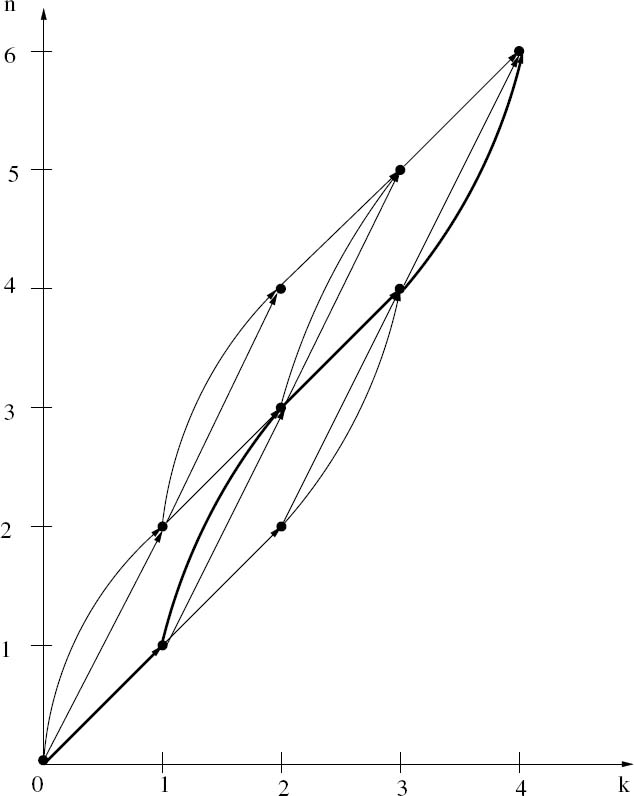
For example, consider a VLC having the alphabet ![]() = {1, 01, 00}, and a sequence of K = 4 source symbols u =(0, 2, 0, 1). This sequence is mapped to a sequence of the VLC codewords c =(1, 00, 1, 01). Its length, expressed in terms of bits, is N = 6. All sequences associated with K = 4 and N = 6 can be represented in the trellis diagram shown in Figure 3.3.
= {1, 01, 00}, and a sequence of K = 4 source symbols u =(0, 2, 0, 1). This sequence is mapped to a sequence of the VLC codewords c =(1, 00, 1, 01). Its length, expressed in terms of bits, is N = 6. All sequences associated with K = 4 and N = 6 can be represented in the trellis diagram shown in Figure 3.3.
In this diagram k denotes the symbol index and n identifies a particular trellis state at symbol index k. The value of n is equivalent to the number of bits of a subsequence ending in the corresponding state. At each node of the trellis, the appropriate match (synchronization) between the received bits and the received symbols is guaranteed.
Note that as the number K of source symbols considered by a symbol-level VLC trellis is increased, its parallelogram shape becomes wider and the number of transitions employed increases exponentially. For this reason, the symbol-level trellis complexity per bit depends on the number K of source symbols considered. In addition to this, the symbol-level trellis complexity depends on the number of entries employed within the corresponding VLC codebook. Furthermore, the difference in length between the longest and shortest VLC codewords influences the symbol-level trellis complexity, since this dictates the size of the acute angles within the symbol-level trellis’s parallelogram shape.
Figure 3.4: Transformed symbol-level trellis for K = 4 and N = 6 using the VLC alphabet ![]() = {1, 01, 00} [40].
= {1, 01, 00} [40].

Let us now introduce the transformation
s = n − klmin
for the sake of obtaining the trellis seen in Figure 3.4, where lmin is the minimum VLC codeword length. The maximal number of states at any symbol index k is
smax = N − Klmin + 1,
which is less than the original trellis of Figure 3.3. Hence the transformed trellis of Figure 3.4 is more convenient for implementation.
3.4.1.2 Bit-Level Trellis
The high complexity of the symbol-level trellis of Section 3.4.1 motivates the use of a bit-level trellis [41], which is similar to that of a binary convolutional code.
The trellis is obtained by assigning its states to the nodes of the VLC tree. The nodes in the tree can be subdivided into a root-node (R) and so-called internal nodes (I) and terminal nodes (T). The root node and all the terminal nodes are assumed to represent the same state, since they all show the start of a new symbol. The internal nodes are assigned one by one to the other states of the trellis. As an example, Figure 3.5 shows the trellis corresponding to the RVLC-2 scheme of {00, 11, 010, 101, 0110}. Figure 3.6 shows two other examples of RVLC trellises.
Figure 3.5: Code tree and trellis for the RVLC-2 scheme of {00, 11, 010, 101, 0110} [42].

Figure 3.6: Bit-level trellises for the Huffman code {00, 01, 11, 100, 101}, and the RVLC-1 {00, 01, 10, 111, 11011}.
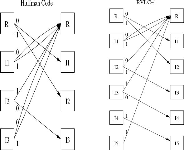
The bit-level trellis of a VLC differs from that of a binary convolutional code in many ways. In the bit-level trellis of a VLC the number of trellis states is equal to the number of internal nodes plus one (the root node), which depends on the specific code tree structure. The maximum number of branches leaving a trellis state is two, corresponding to a separate branch for each possible bit value. Merging of several paths only occurs in the root node, where the number of paths converging at the root node corresponds to the total number of codewords in the VLC. If the variable-length coded sequence consists of N bits, the trellis can be terminated after N sections. Table 3.11 summarizes our comparison of VLCs and convolutional codes. Furthermore, in comparison with the symbol-level trellis, the bit-level trellis is relatively simpler and time invariant. More specifically, as the number of source symbols considered is increased, the number of transitions employed by a bit-level trellis increases linearly, rather than exponentially as in a symbol-level trellis. Note, however, that – unlike a symbol-level trellis – a bit-level trellis is unable to exploit knowledge of the number of transmitted symbols K, even if this is available.
Table 3.11: Comparison of the trellis of a VLC and that of a binary convolutional code

Similar to that for convolutional codes, we may define the constraint length of a VLC. Since a constraint-length-K convolutional code has 2K−1 states in the trellis, the constraint length of a VLC may be defined as
where N is the number of states in the bit-level trellis.
3.4.2 Trellis-Based VLC Decoding
Based on the above trellis representations, either ML/MAP sequence estimation employing the VA [47, 248] or MAP decoding using the BCJR algorithm [48] can be performed. We describe all of these algorithms in the following sections.
3.4.2.1 Sequence Estimation Using the Viterbi Algorithm
Sequence estimation can be carried out using either the MAP or the ML criterion. The latter is actually a special case of the former. The VA [47,248] is invoked in order to search through the trellis for the optimal sequence that meets the MAP/ML criterion. The Euclidean distance is used as the decoding metric for the case of soft decision, while the Hamming distance is used as the decoding metric for the hard-decision scenario.
3.4.2.1.1 Symbol-Level Trellis-Based Sequence Estimation. Consider the simple transmission scheme shown in Figure 3.7, where the K -symbol output sequence u of a discrete memoryless source is first VLC encoded into a N-bit sequence b and then modulated before being transmitted over a channel.
Figure 3.7: A simple transmission scheme of VLC-encoded source information communicating over AWGN channels.

At the receiver side, the MAP decoder selects as its estimate the particular sequence that maximizes the a posteriori probability:
Since the source symbol sequence u is uniquely mapped to the bit sequence b by the VLC encoder, maximization of the a posteriori probability of P(u|y) is equivalent to the maximization of the a posteriori probability of P(b|y), which is formulated as
Using Bayes’s rule, we have

Note that the denominator of (3.14) is constant for all b. Hence, to maximize (3.13) we only have to maximize the numerator of (3.14), and it might be more convenient to maximize its logarithm. Therefore, we have to choose a codeword sequence b that maximizes
If we assume that the channel is memoryless, the first term of (3.15) can be rewritten as

where b = b1b2 · · · b N ; N is the length of the sequence b expressed in terms of the number of bits. Furthermore, assuming that the source is memoryless, then the probability of occurrence P(b) for the sequence b is given by
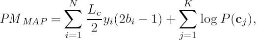
where c1, c2,.. ., cK are the codewords that constitute the sequence b; i.e., we have b =c1c2 · · · cK , and P(cj) is determined by the corresponding source symbol probability. Therefore, based on the channel output and source information, the Path Metric (PM) given by (3.15) is transformed to

Let lj ![]() l(cj) be the length of the codeword cj in terms of bits. Then the branch metric (BM) calculated for the jth branch of the path is formulated as
l(cj) be the length of the codeword cj in terms of bits. Then the branch metric (BM) calculated for the jth branch of the path is formulated as

where we have cj =(cj1 cj2 · · · cjlj), and (yj1 · · · yjlj) represents the corresponding received bits.
Let us detail this algorithm further with the aid of an example. Assume that the source described in Figure 3.7 is a DMS emitting three possible symbols, namely A = {a0, a1, a2}, which have different probabilities of occurrence. Furthermore, the source symbol sequence u is encoded by the VLC encoder of Figure 3.7, which employs the VLC table of C = {1, 01, 00}. Assume that a sequence of K = 4 source symbols u =(0, 2, 0, 1) is generated and encoded to a sequence of VLC codewords c =(1, 00, 1, 01), which has a length of N = 6 in terms of bits. This bit sequence is then modulated and transmitted over the channel. At the VLC decoder of Figure 3.7, a symbol-level trellis may be constructed using the method described in Section 3.4.1.1, which is shown in Figure 3.8. Essentially, the trellis seen in Figure 3.8 is the same as that of Figure 3.3, since we are using the same VLC and source symbol sequence for the sake of comparability. According to Equation (3.19), the branch metric of the MAP Sequence Estimation (SE) algorithm can be readily exemplified, as seen in Figure 3.8 for a specific path corresponding to the VLC codeword sequence c =(1, 00, 1, 01).
For Binary Phase-Shift Keying (BPSK) transmission over a memoryless AWGN channel, the channel-induced transition probability is [8]
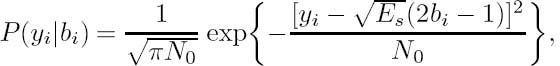
where N0 = 2σ2 is the single-sided power spectral density of the AWGN, σ2 is the noise variance and Es is the transmitted signal energy per channel symbol. Consequently, upon substituting Equation (3.20) into Equation (3.18), the path metric to be maximized is

Figure 3.8: An example of the branch metric calculation for the MAP SE algorithm employed in the VLC decoder of Figure 3.7. The VLC table employed is C = {1, 01, 00}. The transmitted VLC codeword sequence has a length of N = 6 bits, which represents K = 4 source symbols. The received channel observation is y = y1 · · · y6.

Upon removing the common components in Equation (3.21), which may be neglected during the optimization, it can be further simplified to
where

is the channel reliability value.
Correspondingly, the branch metric of Equation (3.19) can be expressed as

If we assume that all paths in the trellis are equiprobable, i.e. the probability of occurrence P(b) of sequence b is equiprobable, then the MAP decoder becomes a ML decoder, and the path metric to be maximized is reduced from the expression seen in Equation (3.15) to
In particular, for BPSK transmission over a memoryless AWGN channel the path metric formulated for the ML decoder is

and the corresponding branch metric is given by

As to hard-decision decoding, the input of the MAP/ML VLC decoder is a bit sequence ![]() . The path metric of the MAP decoder is
. The path metric of the MAP decoder is
In the case of hard decisions and BPSK modulation, a memoryless AWGN channel is reduced to a Binary Symmetric Channel (BSC) having a crossover probability p. Therefore, we have
where h = H(b, ![]() ) is the Hamming distance between the transmitted bit sequence b and the received bit sequence
) is the Hamming distance between the transmitted bit sequence b and the received bit sequence ![]() .
.
Hence, the path metric is formulated as

while the branch metric is given by
As for the ML decoding, assuming that we have 0 ≤ p < 0.5 and all transmitted sequences are equiprobable, the branch metric is simply the Hamming distance between the transmitted codeword and the received codeword, namely H(cj, ![]() j1
j1 ![]() j2 · · ·
j2 · · · ![]() jlj).
jlj).
3.4.2.1.2 Bit-Level Trellis-Based Sequence Estimation. Consider the same transmission scheme as in the symbol-level trellis scenario of Figure 3.7. It is readily seen that the path metric of MAP/ML decoding in the bit-level trellis scenario is the same as that in the symbol-level trellis case, e.g. the path metrics derived in Equations (3.18), (3.22) and (3.26). By contrast, since there is only a single bit associated with each transition in the bit-level trellis, the branch metric is different from that derived for the symbol-level trellis as in Equations (3.19), (3.24) and (3.27). Generally, there are two convenient ways of calculating the branch metric of a bit-level VLC trellis.
For a bit-level trellis each transition ending in the root node represents the termination or completion of a legitimate source codeword, and the merging only occurs at the root node. Hence, for transitions that are not ending at the root node, the source symbol probabilities P(cj) need not to be included in the branch metric. Instead, they are added only when calculating branch metrics for the transitions that do end at the root node.
To be specific, for the soft MAP decoding the branch metrics of the transitions that do not end at the root node of Figure 3.5 are
which may be expressed as

in the case of BPSK transmission over a memoryless AWGN channel. By contrast, the branch metrics of the transitions ending at the root node are
or

in the case of BPSK transmission over a memoryless AWGN channel, where cj is the source symbol corresponding to the transition that ends at the root node.
The second way of calculating the branch metric of a bit-level trellis is to align the source information with each of the trellis transitions. For example, consider the VLC ![]() = {00, 11, 101, 010, 0110} used in Figure 3.5 and assume that the corresponding codeword probabilities are
= {00, 11, 101, 010, 0110} used in Figure 3.5 and assume that the corresponding codeword probabilities are ![]() = {p1, p2, p3, p4, p5}. The probability of the codeword ′010′ being transmitted can be expressed as
= {p1, p2, p3, p4, p5}. The probability of the codeword ′010′ being transmitted can be expressed as
Furthermore, P(′0′), P(′1′/′0′), P(′0′/′01′) can be calculated as the State Transition Probabilities (STPs) of the trellis as defined in [249]. In this example, as seen from the code tree of Figure 3.5, we have


Hence we arrive at

For a generic VLC trellis, the state transition probabilities between two adjacent states associated with an input bit i can be formulated as

where g(sk) represents all the codeword indices associated with node sk in the code tree.
Hence, the branch metric of soft MAP decoding may be expressed as
or

when considering BPSK transmission over a memoryless AWGN channel.
More explicitly, we exemplify this algorithm in Figure 3.9. Consider again the transmission scheme seen in Figure 3.8, except that the VLC decoder employs a bit-level trellis constructed by the method described in Section 3.4.1.2. As seen from Figure 3.9, the branch metrics corresponding to the different state transitions can be readily computed according to Equation (3.42).
For ML soft decoding, source information is not considered, for the sake of reducing complexity. Hence the branch metric is simply expressed as
and we have

for BPSK transmission over a memoryless AWGN channel.
Similarly, for hard-decision decoding, given the crossover probability p, the branch metric of MAP decoding is expressed as
while it is
for ML decoding.
3.4.2.2 Symbol-by-Symbol MAP Decoding
3.4.2.2.1 Symbol-Level Trellis-Based MAP Decoding. In [40] Bauer and Hagenauer applied the BCJR algorithm [48] to the symbol-level trellis in order to perform symbol-bysymbol MAP decoding and hence minimize the SER. The objective of the decoder then is to
Figure 3.9: An example of the branch metric calculation for the bit-level trellis-based MAP SE algorithm employed in the VLC decoder of Figure 3.7. The VLC table employed is C = {1, 01, 00}. The probability P(yi|bi) is the channel-induced transition probability for the ith transmitted bit and the state transition probabilities are defined as ![]()
![]() which can be calculated according to Equation (3.41), given a specific source symbol distribution.
which can be calculated according to Equation (3.41), given a specific source symbol distribution.

determine the APPs of the transmitted symbols uk, (1 ≤ k ≤ K) from the observed sequence y according to
Using Bayes’s rule, we can write

where M is the cardinality of the source alphabet. The numerator of (3.49) can be rewritten as

where sk−1 and sk are the states of the source encoder trellis at symbol indices k − 1 and k respectively, and ![]() k − 1 and
k − 1 and ![]() k are the sets of possible states at symbol indices (k − 1) and k respectively. The state transition of n′ to n is encountered when the input symbol is uk = i. Furthermore, the received sequence y can be split into three sections, namely the received codeword ynn′ + 1 associated with the present transition, the received sequence yn′1 prior to the
k are the sets of possible states at symbol indices (k − 1) and k respectively. The state transition of n′ to n is encountered when the input symbol is uk = i. Furthermore, the received sequence y can be split into three sections, namely the received codeword ynn′ + 1 associated with the present transition, the received sequence yn′1 prior to the
Figure 3.10: A section of transitions from the trellis in Figure 3.3.

present transition, and the received sequence yNn + 1 after the present transition. The received sequence after the split can be seen in Figure 3.10.
Consequently, the probability P(sk − 1 = n′, sk = n, uk = i, y) in Equation (3.50) can be written as

Again, using Bayes’s rule and the assumption that the channel is memoryless, we can expand Equation (3.51) as follows:

The basic operations of the decoder are the classic forward recursion [70] required for determining the values

and the backward recursion [70] invoked for obtaining the values

Both quantities have to be calculated for all symbol indices k and for all possible states n ∈ ![]() k at symbol index k. In order to carry out the recursions of Equations (3.53) and (3.54) we also need the probability
k at symbol index k. In order to carry out the recursions of Equations (3.53) and (3.54) we also need the probability

which includes the source a priori information in terms of the state transition probability P(uk = i, sk = n|sk − 1 = n′) and the channel characteristics quantified in terms of the channel transition probability P(ynn′ + 1|uk = i).
Furthermore, assuming that the source is memoryless, we have

Additionally, for a memoryless channel we can express the channel-induced transition probability seen in Equation (3.55) as the product of the bitwise transition probabilities:

For BPSK transmission over an AWGN channel, the bitwise transition probability is given by [8]

where Es is the transmitted energy per channel symbol and N0 is the single-sided power spectral density of the AWGN.
So far we have obtained all the quantities that we need for computing the APPs of the information symbols uk, which are summarized as follows:

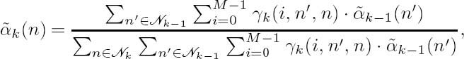
where instead of using αk(n) and βk (n) we used their normalized versions ![]() k(n) and
k(n) and ![]() k(n) to avoid numerical problems such as overflows and underflows. This is because both αk (n) and βk (n) drop toward zero exponentially. For a sufficiently large value of K, the dynamic range of these quantities will exceed the number-representation range of conventional processors. To obtain a numerically stable algorithm, these quantities must be scaled as their computation proceeds. Consequently, the forward recursion
k(n) to avoid numerical problems such as overflows and underflows. This is because both αk (n) and βk (n) drop toward zero exponentially. For a sufficiently large value of K, the dynamic range of these quantities will exceed the number-representation range of conventional processors. To obtain a numerically stable algorithm, these quantities must be scaled as their computation proceeds. Consequently, the forward recursion ![]() k(n) can be written as
k(n) can be written as
with ![]() 0(0) = 1 and k = 1, ..., K, while the backward recursion
0(0) = 1 and k = 1, ..., K, while the backward recursion ![]() k(n) can be expressed as
k(n) can be expressed as

with ![]() K(N) = 1 and k = K − 1, ..., 1.
K(N) = 1 and k = K − 1, ..., 1.
Furthermore, the term in the form of γ(i, n, n′) in Equations (3.59), (3.60) and (3.61) can be computed using Equation (3.55). Note that the scaling or normalization operations used in Equations (3.60) and (3.61) do not affect the result of the APP computation, since they are canceled out in Equation (3.59).
Further simplification of Equation (3.59) can be achieved by using the logarithms of the above quantities instead of the quantities themselves [70]. Let Ak(n), Bk(n) and Γk(i, n′, n) be defined as follows:
and
Then, we have


and

Finally, the logarithm of the a posteriori probability P(uk = m|y) can be written as

The logarithms in these quantities can be calculated using either the Max-Log approximation [250]:

or the Jacobian logarithm [250]:

Figure 3.11: Summary of the symbol-level trellis-based MAP decoding operations.

where the correction function fc(x) can be approximated by [250]

and, upon recursively using g(x1, x2), we have

Let us summarize the operations of the MAP decoding algorithm using Figure 3.11. The MAP decoder processes the channel observation sequence y and the source symbol probabilities P(uk) as its input, and calculates the transition probability Γk(i, n′, n) for each of the trellis branches using Equation (3.67). Then both forward-and backward-recursions are carried out in order to calculate the quantities of Ak(n) and Bk(n) for each of the trellis states, using Equations (3.65) and (3.66) respectively. Finally, the logarithm of the a posteriori probability P(uk = m|y) is computed using Equation (3.68).
3.4.2.2.2 Bit-Level Trellis-Based MAP Decoding. Like the MAP decoding algorithm based on the symbol-level trellis, as shown for example in Figure 3.3, the MAP decoding algorithm based on a bit-level trellis such as that in Figure 3.5 can also be formulated. The forward and backward recursions are defined as follows [42]:

with α0(0) = 1 and α(s ≠ 0) = 0; and

with βN(0) = 1 and βN(s ≠ 0) = 0. Furthermore, we have

where bn is the input bit necessary to trigger the transition from state sn − 1 = s′ to state sn = s. The first term in Equation (3.75) is the channel-induced transition probability. For BPSK transmission over a memoryless AWGN channel, this term can be expressed as [70]

where

is the same for both bn = 0 and bn = 1.
The second term in Equation (3.75) is the a priori source information, which can be calculated using Equation (3.41) of Section 3.4.2.1.2.
According to Equations (3.75) and (3.76), we have

Finally, from Equations (3.73) to (3.78) the conditional Logarithmic Likelihood Ratio (LLR) of bn for a given received sequence y can be expressed as

It is worth noting that the source a priori information and the extrinsic information in Equation (3.79) cannot be separated. A further simplification of Equation (3.79) can be achieved by using the logarithms of the above quantities, as in Section 3.4.2.2.1.
3.4.2.3 Concatenation of MAP Decoding and Sequence Estimation
There are several reasons for concatenating MAP decoding with sequence estimation.
1. For bit-by-bit MAP decoding, the decoder maximizes the a posteriori probability of each bit, which results in achieving the minimum BER. However, the bit-by-bit MAP decoding is unable to guarantee that the output bit sequence will form a valid symbol-based path through the trellis, which implies that there may be invalid codewords in the decoded sequence. Hence MLSE may be performed after the bit-by-bit MAP decoding so as to find a valid VLC codeword sequence. Specifically, given the APPs P(bn|y) provided by the MAP decoder, the sequence estimator selects the specific sequence ![]() that maximizes the probability P(b|y), which is formulated as
that maximizes the probability P(b|y), which is formulated as

2. For symbol-by-symbol MAP decoding, the same problem as outlined above exists. The MAP decoder is capable of guaranteeing that the number of decoded symbols is equal to the number of transmitted symbols and that the corresponding SER is minimized. However, the number of decoded bits may still deviate from that of the transmitted bits. This might be a problem when converting the symbol-by-symbol reliability information to bit-by-bit reliability information. In this case, the MLSE may be performed in order to find a valid path in the trellis. Specifically, given the APPs P(uk|y) generated by the MAP decoder, the sequence estimator selects the specific sequence ![]() that maximizes the probability P(u|y), which is formulated as
that maximizes the probability P(u|y), which is formulated as
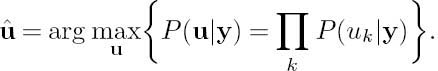
3.4.3 Simulation Results
In this section we characterize the achievable performance of the decoding schemes described in the previous sections.
For all simulations BPSK is used as the baseband modulation scheme and an AWGN channel is assumed. Furthermore, assume that the source is memoryless and it is encoded by the various VLCs [12] as shown in Table 3.12. To be more specific, HUFF represents a Huffman code, RVLC-1 is a asymmetric RVLC having a free distance of 1 and RVLC-2 is a symmetric RVLC having a free distance of 2.
Table 3.12: VLC codes used in the simulations

As we can see, the different source codes have different average codeword lengths; hence for encoding the same source message the resultant bit sequences will have different lengths, which implies that they require different total transmitted signal power. For the sake of fair comparison, we introduce the source code rate Rs, which is defined as

where H(u) is the entropy of the symbol source U, and ![]() is the average codeword length. Consequently, in our simulations Eb/N0 is calculated as
is the average codeword length. Consequently, in our simulations Eb/N0 is calculated as
where Es is the transmitted energy per channel symbol, while M is the number of modulation levels in the signal space of M-ary modulation. For BPSK modulation we have M = 2.
As for our performance measure, we use the so-called Levenshtein SER [40], since, owing to the self-synchronization properties of VLCs, a simple symbol-by-symbol comparison of the decoded sequence with the original sequence is not fair in the context of numerous applications. If a decoding error occurs, there might be VLC symbol insertions or deletions in the decoded sequence. After resynchronization the remaining sequence therefore might be a shifted version of the original one, although a simple symbol comparison would identify the entire remaining part of the sequence as corrupted. A detection metric that is more appropriate in this case is the Levenshtein distance [251], which is defined as the minimal number of symbol insertions, deletions or substitutions that transform one symbol sequence into another. In our simulations we evaluate the SER in terms of the Levenshtein distance.
3.4.3.1 Performance of Symbol-Level Trellis-Based Decoding
In our simulations, six different decoding methods are used, namely MAP/ML sequence estimation using hard decisions (MAP/MLSE-HARD), MAP/ML sequence estimation using soft decisions (MAP/MLSE-SOFT), symbol-by-symbol MAP decoding (SMAP) and symbol-by-symbol MAP decoding concatenated with sequence estimation (SMAP + SE). For every decoding scheme, we use source symbol packets of length K = 100 and transmit 1000 different realizations of the source packets. Furthermore, each of these 1000 packets is transmitted over 50 channel realizations. The simulations are curtailed when all the packets have been transmitted or the number of source symbol errors reaches 5000.
Figure 3.12: SER versus Eb/N0 results for the Huffman code HUFF of Table 3.12, using symbol-level trellis decoding and BPSK transmission over AWGN channels.

Our results for the Huffman code HUFF are shown in Figure 3.12. As we can see, for the Huffman code the performance of soft-decoding schemes is slightly better than that of the corresponding hard-decoding schemes (gain < 0.5 dB). Furthermore, the performance of the MAP decoding scheme is similar to that of the ML decoding scheme, both in the case of soft decoding and for hard decoding. Moreover, the performance of sequence estimation using soft decision is similar to that of the symbol-by-symbol MAP decoding, although the former has a significantly lower complexity. The results of the concatenated MAP decoding and sequence estimation are also shown in Figure 3.12. The concatenation of these two schemes does not affect the achievable SER performance, but it is necessary for solving the previously mentioned length inconsistency problem, namely that the number of decoded bits may be different from the number of transmitted bits.
Our results recorded for the RVLCs RVLC-1 and RVLC-2 scheme of Table 3.12 are shown in Figures 3.13 and 3.14 respectively. In this case it can be seen that the soft-decoding schemes significantly outperform the hard-decoding schemes. More explicitly, RVLC-2 achieves a gain up to 3 dB, as shown in Figure 3.14. By contrast, observe in Figure 3.14 that in the case of hard decision the MAP decoding scheme performs slightly better than ML decoding, while they perform similarly in the case of soft decisions. As in the Huffman coded scenario, the performance of soft sequence estimation is almost the same as that of symbol-by-symbol MAP decoding, as evidenced by Figures 3.13 and 3.14.
Figure 3.13: SER versus Eb/N0 results for the RVLC-1 of Table 3.12, using symbol-level trellis decoding and BPSK transmission over AWGN channels.

Figure 3.14: SER versus Eb/N0 results for the RVLC-2 of Table 3.12, using symbol-level trellis decoding and BPSK transmission over AWGN channels.

The performances of the HUFF, RVLC-1 and RVLC-2 schemes are compared in Figure 3.15. In the case of hard decoding, the RVLC-1 arrangement performs similarly to Huffman coding and slightly better than the RVLC-2 scheme. In the case of soft decoding, the RVLC-2 significantly outperforms both the Huffman code and the RVLC-1 at medium to high SNRs in excess of Eb/N0 > 4 dB. The achievable Eb/N0 gain is as high as about 2 dB ata SERof 10−5.
Figure 3.15: SER versus Eb/N0 performance comparison for HUFF, RVLC-1 and RVLC-2 of Table 3.12, using symbol-level trellis decoding and BPSK transmission over AWGN channels.

3.4.3.2 Performance of Bit-Level Trellis-Based Decoding
In these investigations five different decoding methods are used, namely MAP/ML sequence estimation using hard decisions (MAP/MLSE-HARD), MAP/ML sequence estimation using soft decisions (MAP/MLSE-SOFT) and bit-by-bit MAP decoding concatenated with sequence estimation (BMAP + SE). For each of the decoding schemes, we use the same simulation parameters as those set up for the symbol-level trellis-based decoding described in Section 3.4.3.1.
The results recorded for the Huffman code of Table 3.12 are shown in Figure 3.16. As we can see, for the Huffman code the achievable performance of all decoding schemes is similar.
The corresponding results recorded for RVLC-1 and RVLC-2 of Table 3.12 are shown in Figures 3.17 and 3.18 respectively. This time, the soft-decoding schemes significantly outperform the hard-decoding-aided schemes, especially for the code RVLC-2. The achievable Eb/N0 gain is approximately 2.5 dB at SER = 10−5. In the case of hard decisions, the MAP decoding scheme performs slightly better than the ML decoding scheme, while they perform similarly in the case of soft decisions.
The performances of the Huffman code, RVLC-1 and RVLC-2 are compared in Figure 3.19. In the case of hard decoding the Huffman code performs the best, while in the case of soft decoding the RVLC-1 and RVLC-2 schemes outperform the Huffman code at medium to high channel SNRs in excess of Eb/N0 > 2 dB, and RVLC-2 performs the best. Its gain is as high as about 2 dB at SER = 10−5.
Figure 3.16: SER versus Eb/N0 results for the Huffman code HUFF of Table 3.12, using bit-level trellis decoding and BPSK transmission over AWGN channels.

Figure 3.17: SER versus Eb/N0 results for the RVLC-1 of Table 3.12, using bit-level trellis decoding and BPSK transmission over AWGN channels.
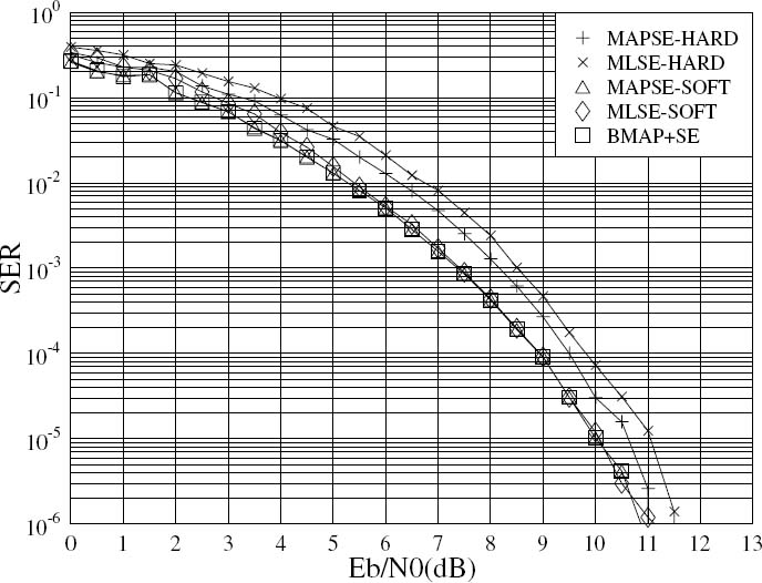
3.4.3.3 Comparison of Symbol-Level Trellis and Bit-Level Trellis-Based Decoding
The achievable performance of various symbol-level trellis-based decoding schemes and those of their bit-level counterparts are compared in Figures 3.20, 3.21 and 3.22 for the Huffman code and the RVLC RVLC-1 and RVLC-2 schemes respectively.
Figure 3.18: SER versus Eb/N0 results for the RVLC-2 of Table 3.12, using bit-level trellis decoding and BPSK transmission over AWGN channels.
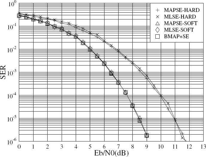
Figure 3.19: SER versus Eb/N0 performance comparison for HUFF, RVLC-1 and RVLC-2 of Table 3.12, using bit-level trellis decoding and BPSK transmission over AWGN channels.

In all of the decoding schemes considered, we assume that the length of the transmitted packets, expressed in terms of bits or symbols as applicable, is known at the decoders. More specifically, the length information includes the number of transmitted bits for the bit-level trellis-based decoding schemes, while both the number of transmitted bits and the number of source symbols has to be known for the symbol-level trellis-based decoding schemes.
Table 3.13: Comparison of various VLC construction algorithms when using the English alphabet as the source

Figure 3.20: SER versus Eb/N0 performance comparison of symbol-level trellis-based decoding and bit-level trellis-based decoding for the Huffman code HUFF of Table 3.12, using BPSK transmission over AWGN channels.

Figure 3.21: SER versus Eb/N0 performance comparison of symbol-level trellis-based decoding and bit-level trellis-based decoding for RVLC-1 of Table 3.12, using BPSK transmission over AWGN channels.

Figure 3.22: SER versus Eb/N0 performance comparison of symbol-level trellis-based decoding and bit-level trellis-based decoding for RVLC-2 of Table 3.12, using BPSK transmission over AWGN channels.

As shown in Figure 3.20, for the Huffman code the symbol-level trellis-based decoding schemes perform slightly better than the bit-level trellis-based decoding schemes, when using soft decoding. However, the above observations are reversed in Figure 3.20 in the case of hard decoding. For the RVLC-1, the symbol-level trellis-based decoding schemes perform slightly better than the corresponding bit-level trellis-based decoding schemes when using hard decoding, while they perform similarly in the case of soft decoding, as seen in Figure 3.21. Finally, for RVLC-2 the symbol-level trellis-based decoding schemes perform consistently better (gain < 0.5 dB) than the corresponding bit-level trellis-based decoding schemes, for both hard decoding and soft decoding.
3.5 Summary and Conclusions
In this chapter we have investigated the design of efficient VLC source codes and their soft decoding methods. After reviewing their construction methods in Section 3.3, we proposed a novel algorithm for the design of efficient RVLCs and VLEC codes in Sections 3.3.4 and 3.3.5 respectively. This optimizes the VLC codeword length distribution on a length-bylength basis. For RVLCs it results in codes of higher efficiency and/or shorter maximum codeword length than the algorithms previously disseminated in the literature, as shown in Tables 3.3, 3.4, 3.5 and 3.9. For VLEC codes, the techniques proposed in Section 3.3.5 significantly reduce the associated construction complexity, as shown in Table 3.10. The optimization procedure is independent of the codeword selection mechanism; therefore, it can be combined with all existing algorithms aiming for efficient codeword design. Our main results are summarized in Table 3.13.
Table 3.14: Summary of ML VLC decoding performance

†The numerical values in this column are the minimum Eb/N0 values required for achieving a SER of 10−5 for the different decoding algorithms.
‡The numerical values in this column are the Eb/N0 gains of soft-decision decoding over the corresponding hard-decision decoding.
In Section 3.4 we considered the soft decoding of VLCs. Both symbol-level trellises and bit-level trellises were described. Based on these trellis representations, two different types of decoding methods – namely sequence estimation using the VA, and MAP decoding employing the BCJR algorithm – were discussed with the aid of a host of simulation results, as shown in Section 3.4.3. Table 3.14 lists some of the ML VLC decoding results.
Based on the simulation results in Table 3.14 and those in Section 3.4.3, we can reach the following conclusions:
- Soft decoding versus hard decoding
At the beginning of Section 3.4 we conjectured that soft decoding may outperform hard decoding according to one of Viterbi’s three lessons [247]. Whether this conjecture is true depends on both the source code and the bit-versus symbol-based trellis structure used. For the Huffman code, soft decoding performs similar to hard decoding in the case of using a bit-level trellis, while soft decoding performs better in the case of symbol-level trellis as evidenced in Figure 3.20. Furthermore, observe in Figures 3.21 and 3.22 that for RVLC-1 and RVLC-2 schemes soft decoding outperforms hard decoding in the case of both trellises. It can be shown that the larger the free distance and the higher the constraint length of the source code, the larger the gain that soft decoding achieves over hard decoding. - MAP versus ML sequence estimation
Our simulation results in Section 3.4.3 show that we cannot attain any performance gain for MAP sequence estimation over ML sequence estimation in the case of soft decoding, although the former exploits the source symbol-probability information. However, in the case of hard decoding MAP sequence estimation achieves some gain over ML sequence estimation for both RVLC-1 and RVLC-2 schemes, as shown in Figures 3.13, 3.14, 3.17 and 3.18.
In addition to the effects of different source codes, Buttigieg [30] investigated the effects of different source statistics on the achievable performance and proposed the so-called MAP factor performance metric. It has been shown that the larger the MAP factor, the larger the attainable Eb/N0 gain [30]. - Bit-level trellis versus symbol-level trellis
Since the symbol-level trellis is capable of exploiting more source information than the bit-level trellis can, the decoding schemes based on a symbol-level trellis are typically capable of performing slightly better than their bit-level counterparts, which can be seen from Figures 3.20, 3.21 and 3.22, as well as Table 3.14. However, according to the construction methods described in Section 3.4.1 the bit-level trellis structure only depends on the specific VLC source code, which is time invariant. By contrast, the symbol-level trellis construction depends on both the specific VLC source code and the specific length of the frame to be decoded; hence it is data dependent. Therefore, the decoding scheme based on the bit-level trellis is typically of lower complexity than that based on the symbol-level trellis. - SE versus symbol-by-symbol MAP decoding
We observed in our investigations that the symbol-by-symbol or bit-by-bit MAP decoding schemes perform similarly to the corresponding SE schemes using soft decisions, as shown in Figures 3.12–3.19. However, the MAP decoding schemes are capable both of exploiting the soft inputs generated by the previous decoding stage and of providing soft outputs, which can be used in a successive decoding stage. These issues will be explored in more detail in the next chapter. - Effect of source codes
In the investigations of this chapter, various source codes have been used, including a df = 1 Huffman code, a df = 1 RVLC and a df = 2 RVLC scheme. It is clear that the free distance of the VLC plays an important role in determining the MAP/ML decoding performance when using soft-decision-based decoding. Our results, seen in Figures 3.15 and 3.19, demonstrate that, as expected, the df = 2 RVLC significantly outperforms the df = 1 RVLC and the Huffman code.
1The number of elements in a set.
2We will also refer to the Buttigieg–Farrell (B–F) divergence distance [29] as the ‘left-aligned common-support distance.’
3The proposed algorithm is also applicable to the construction of the symmetric RVLCs considered in [20].