3.2 Efficient Localized Node-Selection Algorithms
3.2.1 Reformulate the Node-Selection Optimization Problem
We know that when the number of neighbors involved in GOR is given, the denominator of the function ![]() defined in Equation (3.2) is fixed, then maximizing
defined in Equation (3.2) is fixed, then maximizing ![]() is equivalent to maximize its numerator. So we can find the suboptimal solution for each r = 1, 2,
is equivalent to maximize its numerator. So we can find the suboptimal solution for each r = 1, 2,![]() , N, then get a global optimal solution by picking the largest one of the suboptimal solutions. From this analysis, as the packet length Lpkt is fixed, combining Equation (3.1), the optimization problem in (3.3) is equivalent to
, N, then get a global optimal solution by picking the largest one of the suboptimal solutions. From this analysis, as the packet length Lpkt is fixed, combining Equation (3.1), the optimization problem in (3.3) is equivalent to
We now introduce the following corollary that can help us solve this optimization problem more efficiently.
Corollary 3.1 (Local maximum of M(r) is global maximum) Given the available next-hop node set ![]() with
with ![]() , the receiving energy consumption Erx > 0 and transmission energy consumption Etx > 0, the local maximum of the objective function M(r) defined in (3.4) is the global maximum. That is, if M(k − 1) < M(k) and M(k) ≥ M(k + 1) (1 ≤ k ≤ M), M(k) ≥ M(k + n),
, the receiving energy consumption Erx > 0 and transmission energy consumption Etx > 0, the local maximum of the objective function M(r) defined in (3.4) is the global maximum. That is, if M(k − 1) < M(k) and M(k) ≥ M(k + 1) (1 ≤ k ≤ M), M(k) ≥ M(k + n), ![]() 1 ≤ n ≤ M − k.
1 ≤ n ≤ M − k.
Proof. As
![]()
that is
Since EM![]() is concave and positive, we have
is concave and positive, we have
From inequalities (3.5) and (3.6), we have
![]()
that is M(k) ≥ M(k + n), ![]() 1 ≤ n ≤ M − k.
1 ≤ n ≤ M − k.
3.2.2 Efficient Node-Selection Algorithms
3.2.2.1 Algorithm Based on Lemma 2.2 and Corollary 3.1
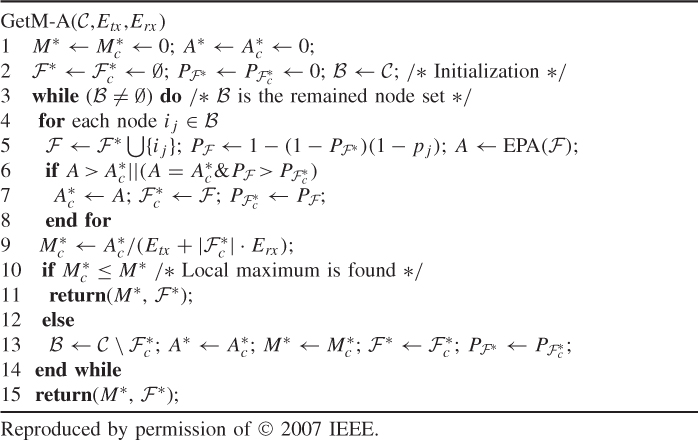
Based on the containing property in Lemma 2.2, a straightforward way to find an optimal node set containing r nodes is to add a new node into the optimal node set containing r − 1 nodes. Furthermore, when a local maximum is found, it is the global maximum based on Corollary 3.1. The algorithm GetM-A in Table 3.1 finds an optimal forwarding candidate set ![]() and the corresponding energy-efficiency value M* of the objective function defined in (3.4). Note that
and the corresponding energy-efficiency value M* of the objective function defined in (3.4). Note that ![]() ,
, ![]() and
and ![]() are all ordered node sets with nodes closer to the destination having higher relay priorities. For feasible sets having the same maximum EPA, we choose the one that achieves higher one-hop reliability (line 6).
are all ordered node sets with nodes closer to the destination having higher relay priorities. For feasible sets having the same maximum EPA, we choose the one that achieves higher one-hop reliability (line 6).
Table 3.1 Pseudocode for finding the maximum energy efficiency value M* and an optimal forwarding candidate set ![]() based on Lemma 2.2
based on Lemma 2.2
It is not difficult to find an algorithm to calculate EPA![]() (in line 5) in
(in line 5) in ![]() running time. Then the algorithm GetM-A costs O(M3) running time in the worst case and in the best case it only costs Ω(M).
running time. Then the algorithm GetM-A costs O(M3) running time in the worst case and in the best case it only costs Ω(M).
Table 3.2 shows the procedure of finding the M* and an ![]() by applying the algorithm GetM-A on the example in Figure 3.1 with Etx = 1 and Erx = 0.5. The procedure runs from Round 1 to Round 3 and in each round it runs from the top to the bottom. In the first round, 〈i1〉 is found as the node achieves the maximum EPA by selecting one forwarding candidate; in the second round, 〈i1, i4〉 is found as the optimal node set by selecting two forwarding candidates; in the third round, 〈i1, i2, i4〉 is found as the optimal node set by selecting three forwarding candidates, and M(3) < M(2); so searching is terminated, and M(2) is the maximum energy efficiency value and 〈i1, i4〉 is an optimal forwarding candidate set.
by applying the algorithm GetM-A on the example in Figure 3.1 with Etx = 1 and Erx = 0.5. The procedure runs from Round 1 to Round 3 and in each round it runs from the top to the bottom. In the first round, 〈i1〉 is found as the node achieves the maximum EPA by selecting one forwarding candidate; in the second round, 〈i1, i4〉 is found as the optimal node set by selecting two forwarding candidates; in the third round, 〈i1, i2, i4〉 is found as the optimal node set by selecting three forwarding candidates, and M(3) < M(2); so searching is terminated, and M(2) is the maximum energy efficiency value and 〈i1, i4〉 is an optimal forwarding candidate set.
Table 3.2 The procedure for finding the maximum energy efficiency value M* and an optimal forwarding candidate set ![]() by applying the algorithm GetM-A on the example in Figure 3.1 with Etx = 1 and Erx = 0.5
by applying the algorithm GetM-A on the example in Figure 3.1 with Etx = 1 and Erx = 0.5

3.2.2.2 Dynamic Programing Algorithm
We now propose another efficient dynamic programing algorithm, which is not based on the containing property, and only costs O(M2) in the worst case and Ω(M) in the best case.
Recall that nodes ij (1 ≤ j ≤ M) in ![]() are ordered according to the advancements as d1 > d2 >…> dM. Denote the set 〈iq, iq+1, …, iM〉 (1 ≤ q ≤ M) as
are ordered according to the advancements as d1 > d2 >…> dM. Denote the set 〈iq, iq+1, …, iM〉 (1 ≤ q ≤ M) as ![]() . Following the denoting,
. Following the denoting, ![]() . According to the relay priority rule in Theorem 2.1 and the definition of EM
. According to the relay priority rule in Theorem 2.1 and the definition of EM![]() , we then have
, we then have
EM![]() (1 ≤ r ≤ M) can be efficiently calculated by applying Equation (3.7) recursively using dynamic programing (Cormen et al. 2001).
(1 ≤ r ≤ M) can be efficiently calculated by applying Equation (3.7) recursively using dynamic programing (Cormen et al. 2001).
The pseudocode of the dynamic programing algorithm GetM-B is given in Table 3.3, where ![]() , F(q, r) is the ordered node set corresponding to EM
, F(q, r) is the ordered node set corresponding to EM![]() , P(q, r) is the corresponding one-hop reliability, and dis are sorted in descending order (d1 > d2…> dM). We also choose the feasible set that achieves a higher one-hop reliability when two feasible sets have the same EPA (line 9). Based on Corollary 3.1, if a local maximum is found (line 16), the searching is terminated and the optimal solution is returned (line 17). The algorithm GetM-B costs O(M2) running time in the worst case and Ω(M) in the best case.
, P(q, r) is the corresponding one-hop reliability, and dis are sorted in descending order (d1 > d2…> dM). We also choose the feasible set that achieves a higher one-hop reliability when two feasible sets have the same EPA (line 9). Based on Corollary 3.1, if a local maximum is found (line 16), the searching is terminated and the optimal solution is returned (line 17). The algorithm GetM-B costs O(M2) running time in the worst case and Ω(M) in the best case.
Table 3.3 Pseudocode of dynamic programming algorithm finding the maximum energy efficiency value M* and an optimal forwarding candidate set ![]()
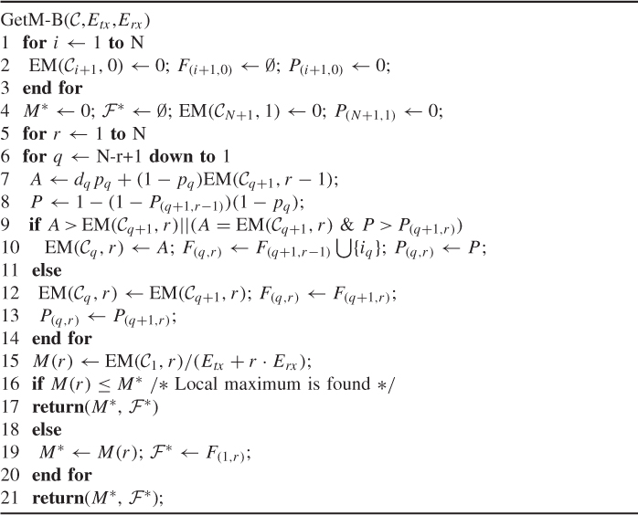
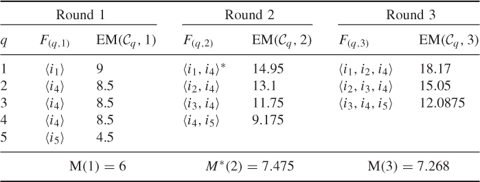
Table 3.4 shows the procedure for finding the M* and an ![]() by applying the algorithm GetM-B on the example in Figure 3.1 with Etx = 1 and Erx = 0.5. The procedure runs from Round 1 to Round 3, and in each round it runs from the bottom to the top. It can be seen that although it finds the same M* (M(2)) and
by applying the algorithm GetM-B on the example in Figure 3.1 with Etx = 1 and Erx = 0.5. The procedure runs from Round 1 to Round 3, and in each round it runs from the bottom to the top. It can be seen that although it finds the same M* (M(2)) and ![]() (〈i1, i4〉) as in Table 3.2, most of the tested node sets are different from the ones in Table 3.2.
(〈i1, i4〉) as in Table 3.2, most of the tested node sets are different from the ones in Table 3.2.
Table 3.4 The procedure for finding the maximum energy efficiency value M* and an optimal forwarding candidate set ![]() by applying the algorithm GetM-B on the example in Figure 3.1 with Etx = 1 and Erx = 0.5
by applying the algorithm GetM-B on the example in Figure 3.1 with Etx = 1 and Erx = 0.5