
2.27. TOTAL SOLUTION OF THE STATE EQUATION
The purpose of this section is to illustrate how one may obtain the complete solution for the output in the time domain of a control system utilizing the state-variable method. In this example, we will want to determine the complete solution by evaluating Eq. (2.255), the state transition equation.
Consider a system described by the following differential equation:
It is desired to determine the output c(t), given that the input r(t) is given by
and the initial conditions are c(0) = 1 and ![]() (0) = 0. The technique employed is to determine the state transition matrix from Eq. (2.256) and then evaluate Eq. (2.255) for x(t). The output c(t) is then evaluated from
(0) = 0. The technique employed is to determine the state transition matrix from Eq. (2.256) and then evaluate Eq. (2.255) for x(t). The output c(t) is then evaluated from
If the state variables are defined by
and u(t) by
u(t) = r(t),
then the system can be described by the following two first-order differential equations:
Therefore, the system can be described by
The state transition matrix, which is defined by Eq. (2.256), can be obtained from Eq. (2.301). We find
From Eq. (2.188), we know that
Therefore,
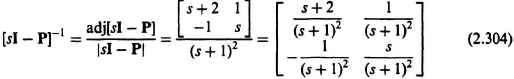
The state transition matrix defined by Eq. (2.256) is the inverse transform of this matrix. It is given by
The full solution for the output can be obtained from Eqs. (2.255) and (2.297) as follows:
Substituting Eq. (2.306) into Eq. (2.307), we obtain the following relationship for the output in terms of the state transition matrix:
We know Φ(t) from Eq. (2.305). We have looked at many similar systems in this chapter, and should know by inspection now that
For this system, the input function u(τ) + ![]() (τ) is obtained as follows:
(τ) is obtained as follows:
Substituting all of these values into Eq. (2.308), we obtain the following expression:

On simplifying, the result becomes
Integrating and simplifying, we finally obtain the output as
We can check the reasonableness of this result by determining the initial value, c(0). Substituting t = 0 into Eq. (2.313), we obtain
which agrees with the value of c(0) specified. It is left as an exercise to the reader to also check that c(0) = 0 which was also specified.