
2.24. DIGITAL COMPUTER EVALUATION OF THE TIME RESPONSE
The state-variable representation of a system’s dynamics easily lends itself to analysis by means of a digital computer. The technique involves the division of the time axis into sufficiently small increments t = 0, T, 2T, 3T, 4T,…, where T is the incremental time of evaluation Δτ. This time increment must be made small enough for accurate results. Round-off errors in the computer, however, limit how small the time increment can be.
To illustrate the procedure, let us consider the equation
By definition of a derivative,
Utilizing this definition, the value of x(t) when t is subdivided into the increments Δτ can be determined. Because Δτ = T, we can say (approximately) that
Substituting Eq. (2.243) into Eq. (2.241), we obtain
Equation (2.244) may be solved for x(t + T) as follows
This equation can be written as
To generalize this expression for the intervals mT, let
where m = 0, 1, 2, 3, 4,.… Therefore, Eq. (2.246) can be written as the recurrence relation
Equation (2.248) states that the value of the state vector at time (m + 1)T is based on the values of x and u at time mT. This resulting recurrence relation is a sequential series of calculations that is very suitable for digital-computer operation. Note that this is a very crude scheme—more sophisticated schemes involve more refined approximations to ![]() [16–18].
[16–18].
To illustrate the capability of using the recurrence equation (2.248), let us evaluate the unit step response of the feedback control system illustrated in Figure 2.29 whose closed-loop transfer function is given by Eq. (2.212). This is the first illustration in this book of developing working digital computer programs to solve problems other than with MATLAB. This program was written using Fortran (FORmula TRANslation) [19]. Several additional problems are solved throughout the book using Fortran and Basic and their corresponding logic flow diagrams, program listings, and program outputs are all illustrated for teaching purposes. In addition, the majority of the solutions in this book are obtained using MATLAB™ (see Section 2.8). The Modern Control System Theory and Design Toolbox, which complements this book, and contains the M-files used for these solutions, is available free from The Math Works, Inc. anonymous FTP server at ftp://ftp.mathworks.com/pub/books/Shinners. (See the Preface for additional information.) MATLAB was used to obtain the graphical results of this problem.
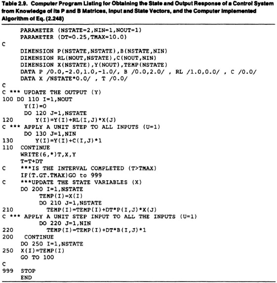
The logic flow diagram for developing the program that can be used to obtain the state responses of second- or higher-order systems as illustrated in Figure 2.34. Table 2.9 illustrates the actual program listing. Figure 2.34 and Table 2.9 should be compared in order to obtain a thorough understanding of the method. This program was then applied to obtain the unit step response of the system illustrated in Figure 2.29 whose phase-variable canonical equations are defined in Eqs. (2.216) and (2.217). The computer output is illustrated in Table 2.10. The results are plotted in Figure 2.35a and b using MATLAB for sampling times T of 0.05 sec (where the response is as expected and very close to the theoretical response, as shown in Figure 2.35b) to 0.5 sec (where an unstable, and obviously erroneous response is indicated). The procedure for obtaining transient responses using MATLAB is described in Section 2.25.
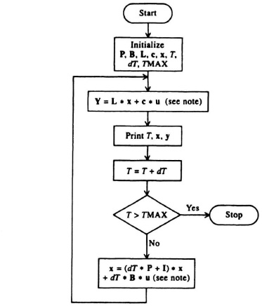
Figure 2.34 Logic flow diagram for obtaining the response time of a control system. Note: For unit step input, u = 1 for all positive time.
Based on the sensitivity of the responses to the sampling time T, a few words of guidance are in order here. In practice, a good guideline is to sample at a rate at least ![]() of the smallest time constant of the system. We will show in Chapter 6 when we discuss the Bode frequency response diagram that this system being analyzed has an approximate bandwidth of 2 rad/sec. Therefore, its time constant is approximately 0.5 sec. As shown in Figure 2.35a, a sampling time of 0.5 sec indicates that it yields an unstable response (although we know that the system response is an exponentially damped sinusoid, and is stable as will be proven in Chapter 4). However, as we increase the sampling rate T, the digital computer result gets better, as illustrated in Figure 2.35a. Using the guideline of sampling at
of the smallest time constant of the system. We will show in Chapter 6 when we discuss the Bode frequency response diagram that this system being analyzed has an approximate bandwidth of 2 rad/sec. Therefore, its time constant is approximately 0.5 sec. As shown in Figure 2.35a, a sampling time of 0.5 sec indicates that it yields an unstable response (although we know that the system response is an exponentially damped sinusoid, and is stable as will be proven in Chapter 4). However, as we increase the sampling rate T, the digital computer result gets better, as illustrated in Figure 2.35a. Using the guideline of sampling at ![]() the system’s time constant, or
the system’s time constant, or ![]() × 0.5 = 0.05 sec, we obtain a quite accurate solution. Figure 2.35a illustrates the improvement as T is decreased from 0.5 to 0.05 sec in incremental steps of DT = 0.5/n, where 1
× 0.5 = 0.05 sec, we obtain a quite accurate solution. Figure 2.35a illustrates the improvement as T is decreased from 0.5 to 0.05 sec in incremental steps of DT = 0.5/n, where 1![]() n
n![]() 10. In Figure 2.35b, the time response obtained using the fast sampling time of 0.05 sec is compared with the theoretical response of the system. The result is very good.
10. In Figure 2.35b, the time response obtained using the fast sampling time of 0.05 sec is compared with the theoretical response of the system. The result is very good.
Notice the accuracy and simplicity of the digital computer’s solution. In addition, the speed of the computer’s solution is of great benefit. Its usefulness as an aid to the control system engineer is quite evident.