
6.9. DIGITAL COMPUTER PROGRAMS FOR OBTAINING THE OPEN-LOOP AND CLOSED-LOOP FREQUENCY RESPONSES AND THE TIME-DOMAIN RESPONSE
For those who do not have access to MATLAB, which has now become an industry standard (more or less), this book also provides other digital computer programs for obtaining the Bode diagram. This approach for providing both MATLAB and other digital computer programs which are not dependent on COTS (commercial-off-the-shelf software) is used throughout this book.
The digital computer is a very valuable tool for computing the gain and phase characteristics as a function of frequency [11, 12]. Several program languages can be used to perform this computation. Perhaps the simplest languages are Basic (Beginner’s All-purpose Symbolic Instruction Code) [13, 14] and Fortran (FORmula TRANslator) [13,14]. Several problems are solved in this chapter and in the rest of this book utilizing these languages with working programs provided. Commercially available computer programs for solving control-system problems are presented in Section 6.21. One of these, MATLAB, has been used for the four illustrative problems shown in Section 6.7, and in Section 6.8 which is dedicated to MATLAB.
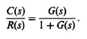
Consider a unity-feedback control system where
It is desired to determine the phase and gain margins of this linear control system, and a Basic program will be utilized in this problem [13, 14]. The coding symbols used are as follows:
W = ω,
G2 = |G(s)|2,
P = phase of G(s),
PM = phase margin,
GOSUB → Compute G2, P.
Figure 6.38 illustrates the logic flow diagram for developing the program that determines the phase and gain margins. Table 6.12 illustrates the actual program. Figure 6.38 and Table 6.12 should be compared in order to obtain a thorough understanding of the method. Table 6.13 illustrates the computer’s output for phase and gain margin. It indicates that unity gain occurs at ω = 31.2 rad/sec where the phase shift is 132.1°. Therefore, the phase margin is 180° − 132.1° = 47.9°. It also indicates that at ω = 95.7 rad/sec, the phase shift is 180°, and the gain margin is 149 dB. To utilize the conventional straight-line asymptotic Bode-diagram technique as a check, Figure 6.39 is drawn. It indicates a phase margin of 48° at a crossover of 31 rad/sec, which is in good agreement. The frequency where 180° phase shift occurs is at 96 rad/sec (compared with 95.7 in the computer run). The gain margin using the straight-line asymptotic curve is only 9 dB and is quite far from the computer run (14.9 dB) because a double break occurs at 100 rad/sec. However, if we correct each of these breaks by the 3-dB error factor, we obtain a gain margin of approximately 15 dB, which is fairly close to the computer solution of 14.7 dB.

Figure 6.38 Logic flow diagram for Bode-diagram analysis.
Table 6.12. Computer Program for Bode-diagram Analysis (Basic program) to Determine Phase and Gain Margins
| LIST 1 REM GEN PHASE AND GAIN MARGIN COMPUTATION FOR GENERAL RESPONSE 10 LET W =.01 20 GOSUB 210 30 IF G2 < = 1 THEN 90 40 IF G2 < = 100 THEN 70 50 LET W = 2 * W 60 GOTO 20 70 LET W = 1.01*W 80 GOTO 20 90 IF P > = 180 THEN 250 100 PRINT “UNITY GAIN,” “W = ” W, “P = ” P 110 LET W = 100*W 120 GOSUB 210 130 IF P < 180 THEN 260 140 LET W = .001*W 150 LET W = 1.01*W 160 GOSUB 210 170 IF P > = 180 THEN 190 180 GOTO 150 190 PRINT “W = ”W,“GAIN MARGIN = ” 4.3429448*LOG(1/G2) 200 GOTO 260 210 LET P= 57.29578*(2*ATN(.01*W) + ATN(.2*W) + ATN(1.5*W)−ATN(.1*W)) 220 LET X= W*W 230 LET G2=99*99*(1 + .01*X)/((1 + .0001*X)↑2*(1 + .04*X)*(1 + 2.25*X)) 240 RETURN 250 PRINT “W=”W, “SYSTEM UNSTABLE” 260 END OK |
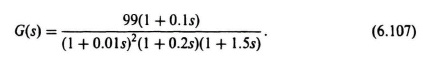
Table 6.13. Phase and Gain Margin Results of Computer Analysis for G(s)H(s) = 99(1 + 0.1s)/[(1 + 0.01s)2(1 + 0.2s)(1 + 1.5s)]
| RUN |
| UNITY GAIN,W = 31.20995 P = 132.1068 |
| W = 95.6849 GAIN MARGIN = 14.8573 OK |
Notice the precision, speed, and simplicity of the digital computer’s solution. Its usefulness as an aid to the control-system engineer is quite evident, and it will be used extensively in this book with either programs presented in this book or MATLAB.
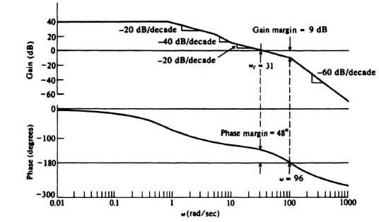
Figure 6.39 Bode-diagram analysis of a unity-feedback system where![]()
We next extend the digital computer as a tool for also determining the open- and closed-loop frequency response, and the time-domain response to a number of standard input signals. Consider a unity-feedback control system where
A Fortran [14–17) program will be utilized in this example in order to determine the open- and closed-loop frequency response, and the Basic [13, 14] program will be utilized to determine the time-domain response.
Figure 6.40 shows the logic flow chart of a Fortran program, called FRECOM, which computes the following relations for various frequencies:
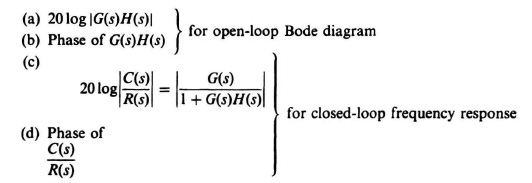
The Fortran program for computing these quantities is shown in Table 6.14 and should be compared with the flow chart of Figure 6.40 to obtain a thorough understanding of the technique. The column labeled “loop again” in Table 6.14 provides the open-loop gain, and the column labeled “response” provides the closed-loop frequency response. Note how simple the complex specification statements become in this language. One should also observe the use of complex function subprograms G(s) and H(s). Once written, the program can now be revised for different systems merely by replacing the two lines containing the arithmetic statements for G and H.

Figure 6.40 Flow diagram FRECOM for computing open- and closed-loop frequency responses.
Table 6.14. Computer Program FRECOM for Determining the Bode Diagram, Open-Loop Frequency Response and Closed-Loop Frequency Response
| COMPLEX S,TFRFCT,LOOPG | |
| COMPLEX G,H | |
| EXTERNAL G,H | |
| COMPLEX TEMP | |
| PRINT *,‘INPUT INITIAL FREQUENCY AND # OF DECADES,’ | |
| READ *,WMIN,JM | |
| PRINT *,WMIN,JM | |
| PRINT *,‘FREQUENCY LOOP GAIN RESPONSE’ | |
| PRINT *,‘RAD/SEC DB DEGREES DB DEGREES‚ | |
| PRINT *,‘⁃⁃⁃⁃⁃⁃⁃⁃⁃⁃⁃⁃ ⁃⁃⁃⁃⁃⁃⁃⁃⁃⁃⁃⁃⁃⁃⁃⁃⁃⁃⁃⁃⁃⁃⁃⁃ ⁃⁃⁃⁃⁃⁃⁃⁃⁃⁃⁃⁃⁃⁃⁃⁃⁃⁃⁃⁃⁃⁃⁃’ | |
| FAC1 =20./ALOG(10.) | |
| FAC2= 180./3.141592654 | |
| WINC=WMIN | |
| DO 1 J-1,JM | |
| IF(J.GT.1)WINC = WMIN*(10**(J−1)) | |
| DO 1 K= 1,9 | |
| W=K*WINC | |
| S=CMPLX(0.,W) | |
| TEMP=G(S) | |
| LOOPG = TEMP*H(S) | |
| TFRFCT=TEMP/(1 + LOOPG) | |
| LOOPG = CLOG(LOOPG) | |
| TFRFCT = CLOG(TFRFCT) | |
| V1 = REAL(LOOPG)*FAC1 | |
| V2 = AIMAG(LOOPG)*FAC2 | |
| V3 = REAL(TFRFCT)*FAC1 | |
| V4 = AIMAG(TFRFCT)*FAC2 | |
| PRINT 900,W,V1,V2,V3,V4 | |
| 900 | FORMAT (F7.2,2X,2F10.2,1X,2F10.2) |
| 1 | CONTINUE |
| STOP | |
| END | |
| COMPLEX FUNCTION G(S) | |
| COMPLEX S | |
| G = 60.*(1. + 0.5*S)/(S*(1 + 5.*S)) | |
| RETURN | |
| END | |
| COMPLEX FUNCTION H(S) | |
| COMPLEX S | |
| H = l. | |
| RETURN | |
| END |
The actual use of the program is extremely simple. During program execution, one enters the starting frequency value and the number of decades of frequency range required. Table 6.15 shows the computer run for the open-(labeled “loop gain”) and closed-loop frequency response (labeled “response”) of this system. Figure 6.41 is a plot of these results. It indicates a phase margin of 74.5° at a gain crossover frequency of 6.4 rad/sec and a closed-loop peaking of 1.8 dB at 2.5 rad/sec. It is immediately evident from examination of the open-loop frequency characteristics that the system is always stable because the phase shift never exceeds −144.87°. Note that the gain margin is infinity because the phase never reaches −180° (except at ω = ∞).
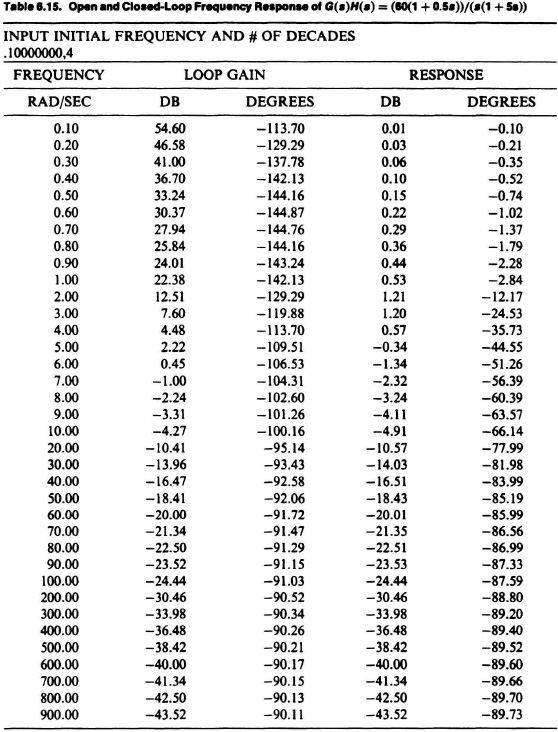
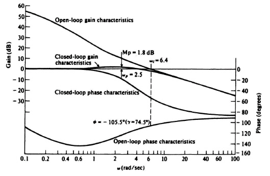
Figure 6.41 Open- and closed-loop frequency response of G(s)H(s) = ![]()
In order to obtain the time-domain response, the differential equations that describe the system must be derived from the given frequency-domain description. Because, in the running example,
![]()
and
H(s) = 1,
then
Upon substitution of G(s) into the expression for C(s)/R(s), the following is obtained:
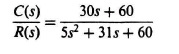
or
C(s)[5s2 + 31s + 60] = R(s)[30s + 60].
This is equivalent to the following differential equation:
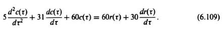
In order to obtain the state equations, let
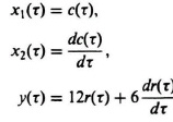
Therefore, Eq. (6.109) is equivalent to the following two first-order differential equations:
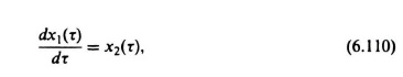

Table 6.16 illustrates the coding of a Basic program called INTER 2, which applies a second-order Runge-Kutta numerical integration method to the solution of two simultaneous differential equations [16, 18, 20]:
Tabla 6.16. Coding of a Basic Program for Solving Two Simultaneous Differential Equations
| STEP 1 | Read in x1(τ0, x2(τ0), τ0,τ, Δ τ τ f Set n = 0, Nmax = |
| STEP 2 | Compute f = f(x1(τn), x2(τn), τn) g = g(x1(τn), x2(τn), τn) |
| STEP 3 | Compute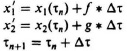 |
| STEP 4 | Compute |
| STEP 5 | Compute |
| STEP 6 | If the final time has not yet been reached, set n = n + 1 and go back to Step 2. Otherwise stop. |
Table 6.16 shows how the values of x1(τ) and x2(τ) are obtained for τ = τ0 = nΔτ, for n = 1, 2, .... A flow chart of the program is shown in Figure 6.42, and the Basic language program is shown in Table 6.17.
In order to use this program, one must define the specific functions f(x1, x2, τ), g(x1, x2, τ), and y(τ) on the specified lines. One must then enter the initial values of τ0, x1(τ0), x2(τ0), and the time increment ∆τ. The tabulation step size is a multiple of ∆τ for which a printout of results is required (this cuts down on a voluminous output).

Figure 6.42 Flow diagram INTER 2 for computing the time-domain response.
Table 6.17. Computer Program INTER 2 for Obtaining the Time-Domain Response
| READY LIST |
|
| 1 | REM THIS ROUTINE APPLIES THE RUNGE-KUTTA METHOD WITH |
| 2 | REM SECOND-ORDER ACCURACY TO THE SOLUTION OF THE |
| 3 | REM SYSTEM OF DIFFERENTIAL EQUATIONS X′ = F(X, Y, T), Y′ = |
| 4 | REM G(X,Y,T) WITH THE INITIAL CONDITIONS X(TO) = X0, Y(TO) = Y0. |
| 5 | REM THE INTEGRATION STEP IS H AND THE SOLUTIONS X(T) AND |
| 6 | REM Y(T) ARE TABULATED ON THE INTERVAL TO < = T < = B IN |
| 7 | REM STEPS OF SIZE L. |
| 8 | REM THE FUNCTIONS F(X,Y,T), G(X,Y,T) ARE ENTERED IN LINES |
| 9 | REM 509 AND 510 RESPECTIVELY AS FOLLOWS: |
| 10 | REM 509 LET F = F(X,Y,T) |
| 11 | REM 510 LET G = G(X,Y,T) |
| 12 | REM THE NUMBERS T0, X0, Y0, B, L, AND H ARE ENTERED AS |
| 13 | REM DATA IN LINE 900. |
| 14 | REM |
| 15 | REM |
| 100 | READ T,X,Y,B,L,H |
| 110 | LET M-INT(L/H) |
| 120 | LET N = INT(B–T)/L) |
| 130 | PRINT “VALUE OF T,” “VALUE OF X,” “VALUE OF Y” |
| 140 | |
| 150 | |
| 160 | PRINT T,X,Y |
| 170 | FOR J = 1 TO N |
| 180 | FOR I = 1 TO M |
| 190 | LET X1 = X |
| 200 | LET Y1 = Y |
| 210 | GOSUB 500 |
| 220 | LET X = X + H*F |
| 230 | LET Y = Y + H*G |
| 240 | LET T = T + H |
| 250 | GOSUB 500 |
| 260 | LET X = (X1 +X)/2 + 0.5*H*F |
| 270 | LET Y = (Y1 + Y)/2 + 0.5*H*G |
| 280 | NEXT I |
| 290 | PRINT, T,X,Y |
| 300 | NEXT J |
| 310 | STOP |
| 500 | LET Y9 = 12 |
| 509 | LET F = Y |
| 510 | LET G = −(31/5)*Y-12*X + Y9 |
| 520 | RETURN |
| 900 | DATA 0,0,1,10,1,0.01 |
| 999 | END |
The solution for a unit step input is shown in Table 6.18. Similarly, the solution for a unit ramp input is shown in Table 6.19. For both cases, the initial input parameters were:
| τ0 = 0 (initial time) | τf = 10 (final time) |
| x1(τ0) = 0 [initial value of x1(τ)] | Δτ = 0.01 (time increment) |
| x2(τ0) = 1 [initial value of x2(τ)] | Δτ′ = 0.5 (tabulation step size) |
Figures 6.43 and 6.44 plot the results of the tabulation in Tables 6.18 and 6.19.

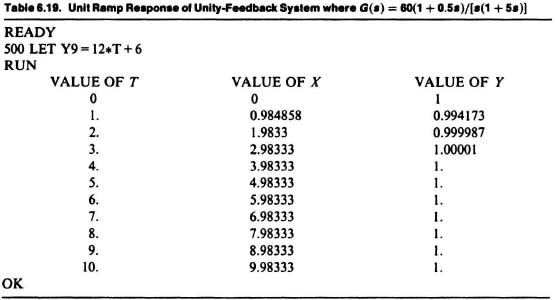
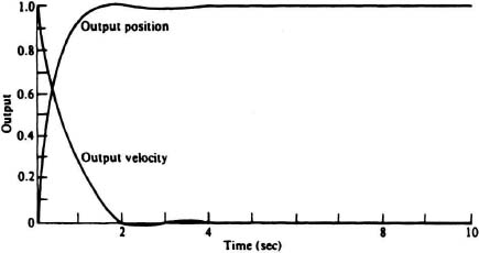
Figure 6.43 Unit step response of unity-feedback system where ![]() .
.
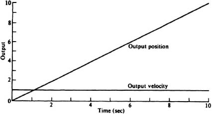
Figure 6.44 Unit ramp response of unity-feedback system where ![]() .
.