
6.8. BODE DIAGRAMS USING MATLAB [7]
In the previous section, several Bode diagrams were illustrated whose amplitude plots were obtained from hand-drawn straight-line asymptotic slopes and whose phase characteristics were calculated from the appropriate trigonometric fucntions. Additionally, several Bode diagrams were also illustrated which were obtained using MATLAB. In this section, the reader will be shown how to obtain the Bode diagrams very easily and accurately using MATLAB.
Let us practice creating Bode diagrams using MATLAB. There are many examples to practice with for creating Bode diagrams on the Modern Control System Theory and Design (MCSTD) Toolbox. Two functions exist that assist in Bode diagrams:
- “bode” returns/plots the Bode response of a system.
- “margins” is described in the MCSTD toolbox. This, in my opinion, has an advantage over the professional version of the Control System toolbox’s “margin” routine. Margins analytically calculates, with analytic precision, the gain and phase margins and their associated frequencies (versus interpolating a single value from a plot).
When trying to find the proper syntax to call the “bode” utility, either use the help feature or look in the reference manual. I personally prefer the help feature, unless I need an example.
Valid syntax for the “bode” utility, for transfer functions, is:
- [mag,phase,w] = bode(num,den)
- [mag,phase,w] = bode(num,den,w)
- [mag,phase] = bode(num,den,w)
- bode(num,den,w)
- bode(num,den)
The left-hand arguments (mag, phase and w) are optional for this function, as described on the second page of the Bode function in The Student Edition book. The result, which can be manually typed, is listed below so that you may try the Bode example in the book:
a = [0, 1; −1. −0.4];
b = [0; 1];
c = [1, 0];
d = 0;
A major short-coming of the Bode diagram is that the margins (gain and phase) are not put onto the plot when it generates the plots. The effect of this is compounded when you want to put them onto the plot, and you discover that you can only modify the phase plot with reasonable ease. Adding to the magnitude plot is almost impossible (prior to MATLAB version 4.0). This is why they have the left-hand arguments, so that you can generate the Bode plots yourself with whatever customization on the plot that you desire. This is what is accomplished in the MCSTD Toolbox when Bode diagrams are obtained in the DEMO, figures, or problems directory.
A. Drawing the Bode Diagram if the System is Defined by a Transfer Function
To illustrate the use of MATLAB for obtaining the Bode diagram, let us consider the following example. The open-loop transfer function of a control system is given by the following:
In order to ease its transformation to MATLAB notation, we multiply all terms in the numerator and denominator as follows:
Therefore, the row matrices for the numerator and denominator are as follows:
num = [0 0 0 1 44 160]
den = [1 1100 180,000 0 0 0].
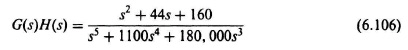
The resulting MATLAB program will first be provided by the listing in Table 6.8, and new commands will then be explained. The resulting Bode diagram is shown in Figure 6.35.
MATLAB and the MCSTD Toolbox automatically select the frequency range used in Figure 6.35 when using the MATLAB program in Table 6.8. If the control-system engineer wants to select a different frequency range, such as from 0.01 to 10,000 rad/sec instead of from 0.1 to 10,000 rad/sec, then we have to use the “log-space” command which is defined as follows:
Table 6.8. MATLAB Program for Obtaining Bode Diagram of System Defined in Eq. (6.106)
| num = [0 0 0 1 44 160]; |
| den = [1 1100 180000 0 0 0]; |
| w = logspace(−2, 4); |
| [mag,ph] = bode(num,den); |
| grid |
| title(‘Bode Diagram of |
| G(s)H(s) = (s + 4)(s + 40)/s^3(s + 200)(s + 900)’) |
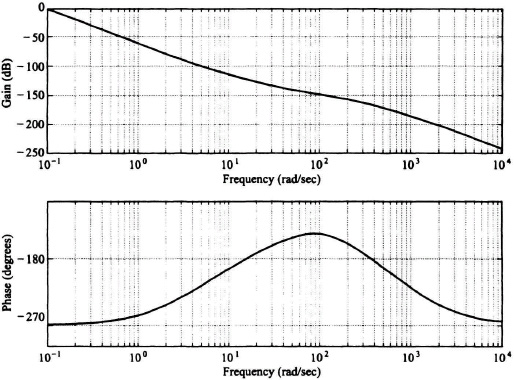
Figure 6.35 Bode diagram for control system whose transfer function is defined by Eq. (6.105).
| w = logspace(−2, 4): | Generates 50 points equally spaced between ω = 10−2 and 104 rad/sec |
In addition, we now have to use the MATLAB command “bode(num,den,w)” which is defined as follows:
| bode(num,den,w): | Generates the Bode diagram from the user-supplied num, den, and the frequency vector w which specifies the frequencies at which the Bode diagram will be calculated. |
Using the MATLAB commands “logspace” and “bode(num,den,w)”, in the MATLAB Program in Table 6.8, is modified as shown in the MATLAB Program in Table 6.9.
Table 6.9. MATLAB Program for Obtaining Bode Diagram of System Defined in Eq. (6.106) with the Logspace Command
| num = [0 0 0 1 44 160]; den = [1 1100 180000 0 0 0]; w = logspace(−2,4); [mag,ph] = bode(num,den,w); grid title (‘Bode Diagram of G(s)H(s) = (s + 4)(s + 40)/s3(s + 200)(s + 900)’) |
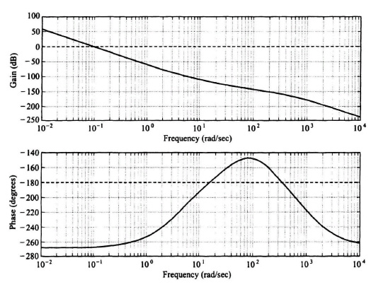
Figure 6.36 Bode diagram of G(s)H(s) = ![]() with the logspace command added.
with the logspace command added.
The resulting Bode diagram is shown in Figure 6.36. Observe that the frequency range of this Bode diagram is 0.01 to 10,000 rad/sec, compared to 0.1 to 10,000 rad/sec in Figure 6.35.
The MCSTD Toolbox command margins provide the following:
‡ gain margin (gm)
‡ phase margin (pm)
‡ frequency (rad/sec) where the phase equals −180° (wcg: ωcg, gain crossover frequency)
‡ frequency (rad/sec) where the gain equals zero dB (wcp: ωcp, phase crossover frequency).
Therefore, adding the following MCSTD Toolbox command to the MATLAB Program in Table 6.9,
[gm, pm, wcg, wcp] = margins(num,den)
will result in the Bode diagram of Figure 6.37 which contains everything previously shown on Figure 6.36 plus the phase margin, the gain margin, the frequency where the gain equals zero dB, and the frequencies where the phase is −180°. Observe from Figure 6.37 that this control system has two gain margins and one phase margin.
Therefore, the MCSTD Toolbox enhances MATLAB. The MCSTD Toolbox DEMO M-file elaborates further on the creation of the Bode diagram with several on-screen examples.
B. Drawing the Bode Diagram if the System is Defined in State-Space Form
The MATLAB command for this case is given by
bode(A,B,C,D).
Figure 6.37 Bode diagram of G(s)H(s) = ![]() with the logspace command added.
with the logspace command added.
As was demonstrated previously in this chapter (e.g., Section 6.6 on the Nyquist Diagram), we must first obtain the state-space form and then use this new command.
To demonstrate this procedure, let us obtain the state-space form from the transfer function given by Eq. (6.106) using the MATLAB command
[A,B,C,D] = tf2ss(num,den)
whose application has been demonstrated earlier in the section on the Nyquist diagram (Section 6.6). The resulting MATLAB program for accomplishing this is shown in the MATLAB program in Table 6.10.
Therefore, the resulting MATLAB program for obtaining the Bode diagram of this problem from the state-space formulation is given by the MATLAB program in Table 6.11. The resulting Bode diagram is identical to that shown in Figure 6.36.

Table 6.11. MATLAB Program for Determining the Bode Diagram from the State-Space Form.
| A = [−1100 − 180000 0 0 0; 1 0 0 0 0; 0 1 0 0 0; 0 0 1 0 0; 0 0 0 1 0] B = [1; 0; 0; 0; 0] C = [0 0 1 44 160]; D = [0]; w = logspace(−2,4); [mag, ph] = bode(A,B,C,D,w) grid title(‘Bode Diagram of G(s)H(s) = (s + 4)(s + 40)/s^3(s + 200)(s + 900)’) |