PROBLEMS

2.1 The periodic function f(t) has the line spectrum shown in Figure P2.1. Assuming that f(t) is an even function, determine the following:

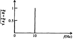
Figure P2.1

(a)  The trigonometric Fourier series for f(t).

(b)  The complex Fourier series for f(t).

2.2. Find v(t) in the circuit of Figure P2.2 using the Laplace transform.

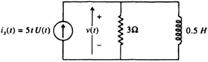
Figure P2.2

2.3. Find x(t) for t0 for

d²x(t)/dt² + x(t) = 0

where x(0) = 1 and dx(0)/dt = −1.

2.4. Consider the Laplace transform

Using the final-value theorem, determine f(∞). Check your answer by finding the inverse Laplace transform f(t) and letting t → ∞.

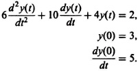
2.5. The initial conditions for the following differential equation

are given by

(a)  Write in its simplest form the Laplace transform of the function Y(s), by taking the Laplace transform of this differential equation.

(b)  Expand Y(s) by means of the partial fraction expansion method. Determine all unknown constants.

(c)  Determine the function y(t) by taking the inverse Laplace transform.

2.6. Repeat Problem 2.5 for the following differential equation and initial conditions:

2.7. Determine the initial and final values of the unit step response of the system of Figure P2.7 using the initial- and final-value theorems, respectively:

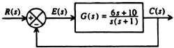
Figure P2.7

2.8. Using the final-value theorem, determine f(∞) for the following function:

2.9 Obtain the inverse Laplace transform for the following expressions:

(a)          

(b)          

(c)          

2.10. Prove that the transfer function for the network illustrated in Table 2.4, item 3, is given by the expression shown.

2.11. Prove that the transfer function for the network illustrated in Table 2.4, item 6, is given by the expression shown.

2.12. Prove that the transfer function for the network illustrated in Table. 2.4, item 9, is given by the expression shown.

2.13. A step input U(t) is applied to a linear system G(s), and the resulting output is given by

(e^−2t − 1)U(t).

Two of these systems are now to be connected in cascade so that the output of the first forms the input to the second. A unit step U(t) is applied to the input of the first system. Determine the output of each system.

2.14. A unit step input U(t) is applied to a linear system G(s) and the resulting output is given by

(1 − e^−4t)U(t).

Determine the transfer function G(s).

2.15. An input tU(t) is applied to a linear system G(s) and the resultant output is given by (1 − 0.5e^−2t − 0.5e^−4t)U(t). Determine the transfer function G(s).

2.16. We wish to determine the transfer function of an element in a control system. Its input, m(t), represents speed, and its output is repreented by y(t). To determine its transfer function, a unit step voltage of 1 volt, corresponding to a speed of 1 ft/sec, is applied to the input, m(t). The output of this element is recorded, and is modeled according to the following equation:

y(t) = (20 − 16e^−2t − 4e^−4t)U(t).

Determine the transfer function, Y(s)/M(s), of this element. Reduce your answer to its simplest form.

2.17. A feedback control system containing four feedback paths is shown in Figure P2.17.

(a)  Draw its signal-flow graph.

(b)  Using Mason’s theorem, determine the transfer function C(s)/R(s).

2.18. Determine the closed-loop transfer function, C(s)/R(s), of the following control system whose signal flow graph is shown in Figure P2.18.

Figure P2.18

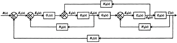
Figure P2.17

2.19. The signal-flow graph of a control system is illustrated in Figure P2.19.

Figure P2.19

Determine the following:

(a)  C(s)/R(s)

(b)  M(s)/R(s)

(c)  C(s)/M(s).

2.20. The signal-flow graph of a control system is represented in Figure P2.20.

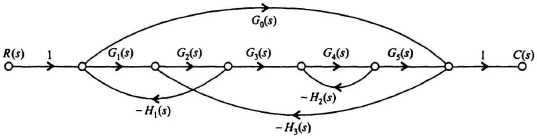
Figure P2.20

(a)  Determine C(s)/R(s).

(b)  Determine E(s)/R(s).

2.21. The signal-flow graph of a feedback control system containing two inputs and two outputs is illustrated in Figure P2.21.

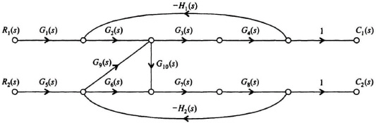
Figure P2.21

(a)  Assuming that R₁(s) = 0, determine C₁(s)/R₂(s) and C₂(s)/R₂(s).

(b)  Assuming that R₂(s) = 0, determine C₁(s)/R₁(s) and C₂(s)/R₁(s).

2.22. The block diagram for the system shown in Figure P2.22 represents the block diagram of one axis of a tracking radar which tries to maintain the actual radar pointing angle C(s) identical to the desired pointing angle R(s). In this block diagram, U(s) represents a wind disturbance which tries to change the actual pointing angle.

(a)  Using Mason’s signal-flow graph method, determine C(s) as a function of R(s) and U(s).

(b)  Repeat part (a) for the transfer function E₁(s)/U(s).

2.23. In the block diagram of the multiple feedback system shown in Figure P2.23, the error function E₁(s) is added directly (through K₁) to the output in order to correct the control system’s output for its error.

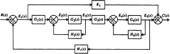
Figure P2.23

(a)  Using Mason’s signal-flow graph method, determine the transfer function C(s)/R(s) for this system.

(b)  Repeat part (a) for the transfer function E₁(s)/R(s).

(c)  Assuming that it is desired to have the output C(s) follow the input R(s), the value of H₁(s) is made equal to 1. If the output C(s) lags behind the input R(s), what should K₁ be made to order to correct the output C(s)?

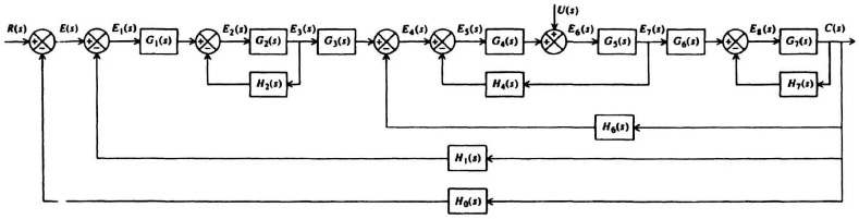
Figure P2.22

2.24. Using signal-flow graphs and Mason’s theorem, find the following for the block diagram shown in Figure P2.24.

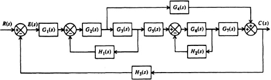
Figure P2.24

(a)  C(s)/R(s)

(b)  E(s)/R(s)

How do the denominators in parts (a) and (b) compare?

2.25. By means of the signal-flow graph and Mason’s theorem, find the transfer function of the closed-loop system, C(s)/R(s), for the block diagram illustrated in Figure P2.25.

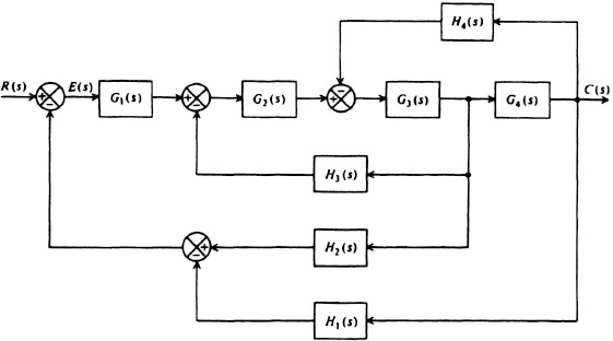
Figure P2.25

2.26. Determine the transfer function of the system shown in Figure P2.25 relating error E(s) and input R(s).

2.27. Determine the transfer function of the overall system shown in Figure P2.27, C(s)/R(s), using the signal-flow graph and Mason’s theorem.

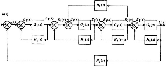
Figure P2.27

2.28. For the control system illustrated in Problem 2.27, determine E₅(s)/E₂(s).

2.29. Repeat Problem 2.27 with the feedback path containing element H₅(s) removed.

2.30. Determine the transfer function of the system shown in Figure P2.27 relating error E(s) and input R(s).

2.31. Repeat Problem 2.30 with the feedback path containing element H₅(s) removed.

2.32. Determine the transfer function of the overall system shown in Figure P2.32, C(s)/R(s), using the signal-flow graph and Mason’s Theorem.

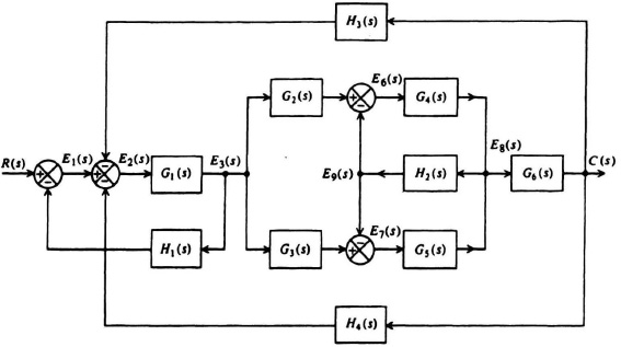
Figure P2.32

2.33. Determine the transfer function of the system shown in Figure P2.32 relating error E₁(s) and input R(s).

2.34. Repeat Problem 2.32, with the feedback path containing element H₁(s) removed.

2.35. The block diagram of an antenna positioning control system is represented by the block diagram in Figure P2.35. The disturbance, D(s), represents an external disturbance in the form of wind gusts that hit the antenna. The feedforward transfer function, G_d(s), is used to eliminate the effect of the disturbance D(s) on the output, C(s). Assume that R(s) = 0.

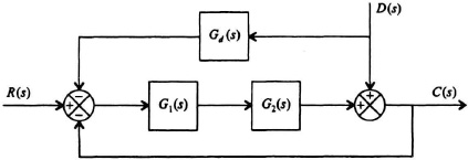
Figure P2.35

(a)  Determine the transfer function C(s)/D(s).

(b)  Determine the explicit transfer function G₄(s) which will eliminate the effect of D(s) on C(s).

2.36. The two-feedback loop control system illustrated in Figure P2.36 is to be designed so that the inner feedback loop has zero effect (the inner feedback loop’s transfer function, G(s)H(s), approaches zero) at very low and very high frequencies.

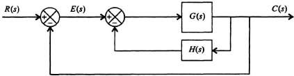
Figure P2.36

When the open-loop transfer function, G(s)H(s), approaches zero at very low and very high frequencies, C(s)/E(s) becomes approximately equal to G(s). Assume that the transfer function of G(s) is given by:

Determine the transfer function of H(s) in the inner feedback loop so that the inner feedback loop has zero effect at very low and very high frequencies.

2.37. Repeat Problem 2.33, with the feedback path containing element H₁(s) removed.

2.38. Determine the system transmission T(s) = C(s)/R(s) for the signal-flow graph shown in Figure P2.38.

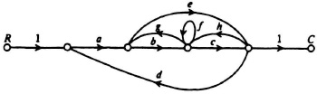
Figure P2.38

2.39. Synthesize a signal-flow graph for the following source-to-sink transmission T(s), such that each branch transmission in the graph is a different letter (each branch transmission is a function of s ):

2.40. Synthesize a signal-flow graph for the following source-to-sink transmission expression, such that each branch transmission in the graph is a different letter (each branch transmission is a function of s):

2.41. The signal-flow graph of a control system is illustrated in Figure P2.41.

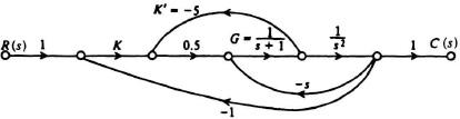
Figure P2.41

(a)  Determine the overall transmission T(s) = C(s)/R(s).

(b)  If the K′ branch were made zero, the same overall transmission could be obtained by appropriately modifying the G(s) branch. Determine the required modification.

2.42. Determine the phase-variable canonical form for the systems characterized by the following differential equations:

(a)          

(b)          

(c)          

(d)          

2.43. The approximate linear equations for a spherical satellite are given by

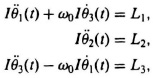
where θ₁(t), θ₂(t), θ₃(t) represent angular deviaitons of the satellite from a set of axes with fixed orientation, L₁, L₂, L₃ represent applied torques, I represents the moment of inertia, and ω₀ represents the angular frequency of the oriented axis. Determine the phase-variable canonical form of the system’s dynamics.

2.44. The signal-flow graph of Figure P2.44 illustrates the process of interest accrual in a savings account. The initial deposit is represented as r(t) and the total savings is represented as c(t). The interest is assumed to be a constant of K% per year. It is interesting to note from this representation that it represents a positive feedback process.

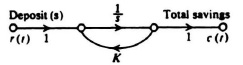
Figure P2.44

(a)  Write the state equation of this system and determine the total savings as a function of deposit(s) and the interest rate.

(b)  Compare the total savings at the end of a 10-year period for the following two conditions:

1. An initial deposit of $10,000 held in a savings account over a 10-year period.

2. A yearly deposit of $1000, totalling $10,000 over a 10-year period, in a savings account.

In each case assume that the interest rate K is 5% per year.

(c)  How do each of these cases compare with the case of savings without interest?

2.45. The voltage buildup of a simple electronic oscillator is given by the Van der Pol equation as follows:

Determine the state equations.

2.46. The Apollo 11 mission, in which astronauts Neil Armstrong and Edwin Aldrin successfully soft landed the Lunar Excursion Module (LEM) on the lunar surface, was a historic event. Figure P2.46a is a photograph of the LEM vehicle taken by astronaut Michael Collins from the Apollo Command Module window after they separated. In order to obtain the state-variable vector equations of the LEM during the terminal soft-landing phase, let us consider the basic physics involved [24]. Figure P2.46b illustrates the forces acting on the LEM, assuming that the vehicle is vertical and subject to the following conditions:

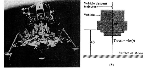
Figure P2.46 (a) Apollo 11 astronauts Neil Armstrong and Edwin Aldrin are inside the Lunar Excursion Module (LEM) separated from the Apollo command module. (Official NASA photo) (b) Forces acting on LEM.

(a)  The only forces acting on the vehicle are its own weight and the thrust which acts as a braking force.

(b)  The moon is flat in the vicinity of the desired landing point.

(c)  The propulsion system is capable of producing a mass flow rate (t)

Based on these assumptions, the motion of the vehicle is governed by the following relation:

where

 x(t) = altitude,

m(t) = total mass

(t) = mass flow rate0,

     g = acceleration of gravity at the surface,

     K = velocity of exhaust gases = constant > 0.

Defining the state variables as

x(t) = x₁(t),   x₂(t) = (t)
x₃(t) = m(t),   u₁(t) = (t),

determine the phase-variable canonical equation of the system during the terminal soft-landing phase of the mission.

2.47. Determine the phase-variable canonical equation for the system shown in Figure P2.47.

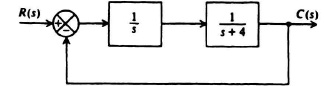
Figure P2.47

2.48. The landing of an aircraft consists of several phases [25]. First, the aircraft is guided towards the airport with approximately the correct heading by radio direction-finding equipment. Within a few miles of the airport, radio contact is made with the radio beam of the instrument landing system (ILS). In following this beam, the pilot guides the aircraft along a glide path angle of approximately 3° towards the runway. Finally, at an altitude of approximately 100ft, the flare-out phase of the landing begins. During this final phase of the landing, the ILS radio beam is no longer effective, nor is the −3° glide path angle desirable from the viewpoint of safety and comfort. Therefore, the pilot must guide the aircraft along the desired flare path by making visual contact with the ground. Let us consider, in this problem, the states of the aircraft during the final phase of the landing (the last 100 ft of the aircraft’s decent). Figure P2.48a defines the aircraft’s coordinates and angles. Figure P2.48b illustrates the aircraft’s block diagram in terms of measurable state signals from the elevator deflection angle δ_e to the altitude h(t). The state signals being fed back are all measurable. For example, the altitude h(t) can be measured with a radar altimeter, and the rate of ascent (t) can be measured with a barometric ratemeter. In addition, the pitch angle θ(t) and the pitch rate (t) can be easily measured using gyros. Defining the states of the aircraft-landing system as

x₁(t) = (t),    x₂(t) = θ(t),

x₃(t) = (t),    x₄(t) = h(t),    u_l(t) = δ_e(t),

determine the phase-variable canonical equation of this system.

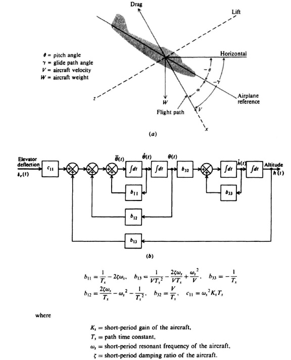
Figure P2.48

2.49. Determine the phase-variable canonical equation for the system shown in Figure P2.49.

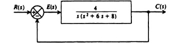
Figure P2.49

2.50. A finless torpedo is directionally unstable without control. However, its controlled performance is usually made better than that of a torpedo with fins by utilizing optimal control theory. It is possible to synthesize an intercept trajectory that overcomes the problems associated with random disturbances, measurement noise, and drift [26]. Figure P2.50 illustrates the motion of such a torpedo in the yaw axis. If it is assumed that the optimal intercept trajectory is a straight line, then the usual small-angle assumptions are reasonably accurate and the problem can be treated by linear techniques. The following equations describe yaw acceleration (t), sideslip effects (t), and the command input δ_c(t), for the finless torpedo:

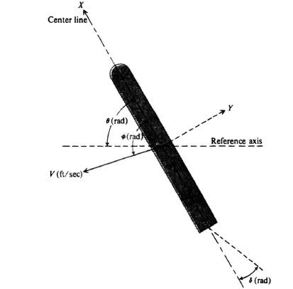
Figure P2.50

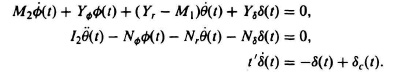
The value t′ is a normalized time parameter. Because the problem has been presented on the assumption that only small perturbations are being considered, no bounds need to be placed on δ_c(t). Determine the state equation in matrix/vector form for this system with the coefficients, normalized with respect to ship length, defined as follows:

M₁ = longitudinal virtual mass coefficient= 1.56,

M₂ = lateral virtual mass coefficient = 2.92,

  I₂ = virtual moment of inertia cofficient = 0.138,

  = static side force rate coefficient = 0.60,

= static yaw moment rate coefficient = 0.99,

  Y_r = damping force rate coefficient = 0.20,

  N_r = damping moment rate coefficient = −0.08,

  Y_δ = rudder force rate coefficient = 0.10,

  N_δ = rudder moment rate coefficient = Y_δe_R = −0.50

   e_R = dimensionless coordinate of rudder side force = −0.50.

2.51. Given

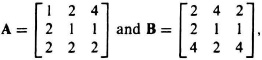
determine AB⁻¹. How can you check your results?

2.52. Determine the state and output equations for the system shown in Figure P2.52.

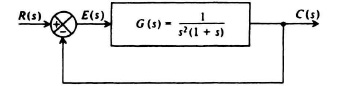
Figure P2.52

2.53. Determine the state and output equations for an open-loop system where

2.54. Repeat Problem 2.53 with

2.55. Repeat Problem 2.53 with

2.56. Determine the state-variable signal-flow graph and the state and output equations for the following open-loop system:

2.57. The automatic depth control of a submarine is an interesting control problem. Figure P2.57a illustrates a representative problem, where the actual depth of the submarine is denoted as C(s). In practice, the actual depth of a submarine is measured by a pressure transducer. This measurement is then compared with the desired depth R(s). Any differences are amplified in a control system which appropriately adjusts the stem plane actuator angle θ. An equivalent block diagram of such a system is illustrated in Figure P2.57b. Determine the state-variable signal-flow graph and the state and output equations for this system.

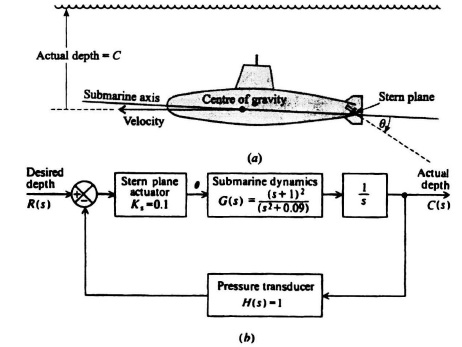
Figure P2.57

2.58. Determine the vector-matrix form of the following set of first-order differential equations:

2.59. Control techniques are being utilized to solve problems in the aquatic systems field. These ecological problems require a mathematical model to provide an understanding of the characteristics within the system. An aquatic ecosystem model [27] for Lago Pond, a Georgia farm pond, has been developed. This pond is a man-made pond created by an earth-fill dam and is used for sport fishing. The pond is fertilized in the spring and periodically throughout the summer in order to cause algal blooms; this increase in primary productivity travels up the food chain and causes an increase in the fish population. A constant coefficient model of Lago Pond, which assumes a constant temperature environment, is given by the following set of equations:

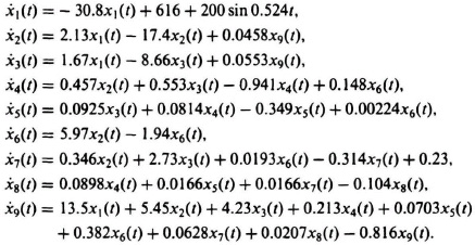
The states x₄(t), x₅(t), x₆(t), and x₇(t) represent the levels of redbreast, warmouth, chaoborus, and bluegill sunfish in the lake; the state x₈(t) represents the level of bass in the lake. States x₁(t), x₂(t), and x₃(t) represent nutrient factors for the fish as a result of pond fertilization, and state x₉(t) represents detritus (rocks and other small material worn or broken away from a mass due to the action of water).

(a)  Determine the companion matrix P, and Bu(t), for the state equation of the system:

(t) = Px(t) + Bu(t).

(b)  Simulate this constant coefficient model of Lago Pond on a digital computer, and determine the time responses of the states for 12 months using the algorithm given in Section 2.24 (see Eq. 2.248). Assume the following initial conditions for the nine states (units are in Kcal/m²): x₁ = 20; x₂ = 3.5; x₃ = 6.4; x₄ = 7.16; x₅ = 3.44; x₆ = 10.8; x₇ = 61; x₈ = 16.5; x₉ = 400. What conclusions can you reach from your results?

2.60. Determine the phase-variable canonical form of the state and output vector equations for the following system, where r(t) represents the reference input and n(t) represents the noise entering the system:

2.61. Determine the phase-variable canonical state and output equations for the control system of Figure P2.61 from knowledge of the system’s transfer function.

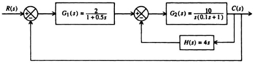
Figure P2.61

2.62. A control system has a transfer function given by

(a)  Derive the state-variable signal-flow graph for this control system. Label the states on this diagram.

(b)  Determine the phase-variable canonical state and output equations from the state-variable signal-flow graph of part (a).

2.63 The closed-loop transfer function of a control system is given by the following:

(a)  Determine and illustrate the state-variable signal-flow graph of this system.

(b)  Find the state and output equations of this system from the state-variable signal-flow graph.

(c)  Write the phase-variable canonical form of the system’s equations.

2.64. Determine analytically the state transition matrix of the system considered in Problem 2.56.

2.65. Determine the state transition matrix of the following open-loop control system analytically:

2.66. Repeat Problem 2.65 with

2.67. A nuclear reactor has been operating in equilibrium for a long period of time at a high thermal-neutron flux level, and is suddenly shut down. At shutdown, the density of iodine 135 (I) is 5 × 10¹⁶ atoms per unit volume and that of xenon 135 (X) is 2 × 10¹⁵ atoms per unit volume. The equations of decay are given by the following state equations:

(a)  Determine the state transition matrix using Eq. (2.256).

(b)  Determine the system response equations, I(t) and X(t).

(c)  Determine the half-life time of I 135. The unit of time for and is hours.

2.68. Determine whether the following matrices can represent state transition matrices by checking whether they satisfy all of the necessary properties to be a state transition matrix:

(a)

(b)

2.69. Control-system concepts have recently been applied in attempts to solve some problems of sociology and of economics. Let us consider one such example concerned with the problem of underdeveloped countries [28, 29]. Representing the number of underdeveloped countries by C_u, and developed countries by C_d, the state variable x₁ is defined as

x₁ = C_u/C_d.

The state variable x₁ is an indication of the development of the countries in the world. A second state variable x₂ is used to represent the tendency towards underdevelopment. In writing a set of dyamical equations for these state variables, it is important to recognize that the tendency towards under-development can be reduced by means of technical-assistance programs, education, etc. However, it is interesting to note that studies indicate that the gap between the developed and underdeveloped nations is growing, because the underdeveloped nations tend to remain in their present state relative to the developed area [29]. It has been proposed that the following set of state equations may be used to represent this process [28]:

(a)  Determine the state transition matrix of this system from the state-variable signal flow graph when A = 4, B = C = 1, and D = 2.

(b)  Determine the response of this system when x₁(0) = 2 and x₂(0) = 1.

2.70. Determine the state transition matrix of the following open-loop control system analytically:

2.71. The effectiveness of a mass-marketing campaign to sell a product can be predicted by analyzing its state-equation representation using control techniques. Consider the promotion of a new automobile in a city by the mass media including television, radio, newspapers, and periodicals. Consider the population under study to be made up of the following three groups:

x₁(t) represents the group who might by receptive to the automobile;

x₂(t) represents the group who buys the automobile;

x₃(t) represents the group removed from groups x₁(t) and x₂(t) due to death or other factors that cause them to be isolated or removed from the groups x₁(t) and x₂(t).

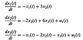
The rate at which new receptives are added to the population is equal to u₁(t), and the rate at which new buyers are added to the population is equal to u₂(t). The model of this system can be represented by the following set of equations:

Assume a closed population model (u₁(t) = u₂(t) = 0).

(a)  Determine the state transition matrix of this system when m = 4, n = 2, and p = l.

(b)  Forecast how well the automobile will sell and whether the marketing campaign will be successful by determining the response of x₂(t) of this system for the following initial conditions: x₁(0) = 100,000; x₂(0) = 20,000; x₃(0) = 2000. What conclusions can you reach from your results? The unit of time is in weeks.

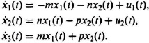
2.72. A very interesting ecological problem is that of rabbits and foxes in a controlled environment. If the number of rabbits were left alone, they would grow indefinitely until the food supply was exhausted. Representing the number of rabbits by x₁(t), their growth rate is given by

(t) = Ax₁(t).

However, rabbit-eating foxes in the environment change this relationship to the following:

(t) = Ax₁(t) − Bx₂(t),

where x₂(t) represents the fox population. In addition, if foxes must have rabbits to exist, then their growth rate is given by

(t) = −Cx₁(t) + Dx₂(t),

(a)  Assume that A = 1, B = 2, C = 2, and D = 4. Determine the state transitions matrix for this ecological model.

(b)  From the state transition matrix, determine the response of this ecological model when x₁(0) = 100 and x₂(0) = 50. Explain your results.

2.73. [30] A very important ecological control problem is the treatment of wastes in water. Control engineers are attempting to solve this problem by adding bacteria, which grow by using the pollutant as a nutrient, to the waste flow. In this manner, wastes in sewage treatment plants can be eliminated by this natural biological process. Microbial growth models currently being used to analyze this kind of problem are based on differential equations. Defining x(t) as the bacteria concentration required for pollutant removal, s(t) as the pollutant serving as the nutrient substance for the bacteria, and D as the rate of flow/volume (dilution rate), the normalized material balance equations can be approximated by the following two state equations:

(t) = ux(t)− Dx(t)

   (t) = −ux(t) − Ds(t).

(a)  Assuming that the specific growth rate u is a constant, determine the state transition matrix of this ecological control system.

(b)  Analyze the meaning of the state transition matrix obtained for this problem. Under what conditions does a balance exist in this ecological control system?

2.74. Substances x₁(t) and x₂(t) are involved in the reaction of a chemical process. The state equations representing this reaction are as follows:

(t) = −8x₁(t) + 4x₂(t),

(t) = 4x₁(t) − 2x₂(t).

(a)  Determine the state transition matrix of this chemical process.

(b)  Determine the response equations of this system, x₁(t) and x₂(t) when

x₁(0) = 2,

x₂(0) = 1,

(c)  At what value of time will the amount of substances x₁(t) and x₂(t), be equal? The unit of time for x₁(t) and x₂(t) is hours.

2.75. Substances x₁(t) and x₂(t) are involved in the reaction of a chemical process. The state equations representing this reaction are as follows:

   (t) = −4x₁(t) + 2x₂(t),

(t) = 2x_l(t) − x₂(t).

(a)  Determine the state transition matrix of this chemical process.

(b)  Determine the response of this system when:

x₁(0) = 200,000 units,

x₂(0) = 10,000 units.

(c)  At what value of time will the amount of substances x₁(t) and x₂(t) be equal?

2.76. The state equations of a chemical process which mixes chemicals x(t) and y(t) are given by the following:

(t) = −100x(t),

      (t) = −10x(t) + 2y(t).

The initial conditions of states x(t) and y(t) are as follows:

x(0) = 1000,

y(0) = 4000.

(a)  Determine the state transition matrix.

(b)  Determine the system’s response equations x(t) and y(t).

(c)  Find the time it takes in minutes for element x(t) to decay to 200 units. (The unit of time for x(t) and y(t) is hours.)

2.77. (a) Determine the state transition matrix of the control system of Figure P2.77 analytically from the definition of the state transition matrix.

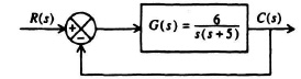
Figure P2.77

(b)  If the initial position and velocity of the system are 10 units and 20 units/sec, respectively, determine the system response equations for position and velocity: c(t) and (t).

2.78. (a) Determine the state transition matrix for a system whose companion matrix P is given by

Use the definition of the state transition matrix as given by Eq. (2.256).

(b)  Solve the state transition equation, Eq. (2.255), for the system whose P matrix is given in part (a). Assume that the input is a unit step function, its input vector, B, is given by

and the initial state vector, x(0), is given by

2.79. Repeat Problem 2.78 if the P matrix is changed to the following.