
2.30 ILLUSTRATIVE PROBLEMS AND SOLUTIONS
This section provides a set of illustrative problems and their solutions to supplement the material presented in Chapter 2.
I2.1. Determine the poles and zeros of
![]()
SOLUTION: Simple poles are located at s = 0, −2, −6
Pole of order two located at −8
Simple zeros located at −1, −4
I2.2. Determine the Laplace transform of f(t) which is given by
f(t) = te4t, t ≥0
f(t) = 0, t > 0.
SOLUTION: From Appendix A, eighth item: For n = 2 and a = −4, we obtain
![]()
I2.3. Determine the Laplace transform F(s) for the function f(t) illustrated:

Figure I2.3
f(t) = 2U(t) − 4U(t − 1) + 2U(t − 2)
From Table 2.1, item 2, and the time-shifting theorem, we obtain

I2.4. Determine the initial value of c(t) where the Laplace transform of C(s) is given by:
![]()
SOLUTION: From the initial-value theorem
![]()
we obtain,
![]()
I2.5. Determine the final value of c(t) when the Laplace transform of C(s) is given by
![]()
SOLUTION: From the final-value theorem
![]()
we obtain,

I2.6. Determine the final value of c(t) when the Laplace transform of C(s) is given by
![]()
SOLUTION: The final-value theorem cannot be applied in this problem because the function sC(s) is not analytic in the right half-plane.
I2.7. Determine the Laplace transform of
c(t) = sin ωt U(t − 2)
from knowledge of the Laplace transform of a sine wave (see Table 2.1, item 7) and the time-shifting theorem.
SOLUTION:
![]()
I2.8. Determine the Laplace transform of
c(t) = e−3t sin ωt U(t)
from knowledge of the Laplace transform of a sine wave (see Table 2.1, item 7) and the frequency-shifting theorem.
SOLUTION:
![]()
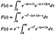
I2.9. Determine the Laplace transform of the function f(t) where
f(t) = e−t(t−1)U(t − 1).
SOLUTION:
![]()
To integrate this equation, it is necessary to change the variable as follows:
Therefore,
Adding the term
e0.52 e(s+1)2
inside and outside the integral to complete the square, we obtain the following:
![]()
Let us now change the variable. By defining the new variable T as follows:
T = τ + 0.5(s + 1).
Therefore,
![]()
The integral term is equal to:
0.5π0.5(1 − error function)
Abbreviating the error function as “erf,” the Laplace transform is given by the following:
F(s) = 0.5π0.5e0.52(s−1)2(1 − erf(0.5)(s + 1)).
I2.10. Determine the residues of F(s) where
![]()
which has single poles at s = −2 and s = −4.
SOLUTION: The residue at s = −2 is given by
![]()
The residue at s = −4 is given by
![]()
I2.11. Determine the inverse Laplace transform of C(s) where
![]()
SOLUTION: Using partial-fraction expansion, we obtain the following:
![]()
where
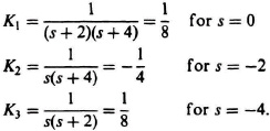
From Table 2.1, items 2 and 6 we obtain the following:
![]()
I2.12. Determine the inverse Laplace transform of C(s) where
![]()
SOLUTION: Using partial-fraction expansion, we obtain the following:
![]()
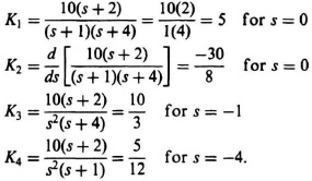
From Table 2.1, items 2, 3, and 6, we obtain the following:
![]()
I2.13. Determine the value of c(t) for the following differential equation using the Laplace transform. Assume that the initial conditions are zero, and U(t) represents a unit step.
![]()
SOLUTION:
Using partial-fraction expansion, we obtain the following:
![]()
where

c(t) = (0.1e−t + 0.067e−6t − 0.167e−3t)U(t).
I2.14. Solve the following two differential equations for x1(t) and x2(t) by means of the Laplace transform.
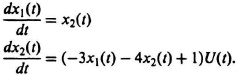
The initial conditions are: x1(0) = 1; x2(0) = 0.
SOLUTION:
Therefore,
sX1(s) − 1 = Xs(s).
Solving for X1(s):
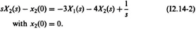
Substituting X1(s) from Eq. (I2.14-3) into Eq. (I2.14-2), we obtain:
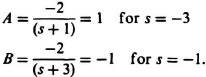
Using partial-fraction expansion, we obtain:
![]()
where
![]()
Taking the inverse Laplace transform of X2(s), we obtain
x2(t) = (e−3t − e−t)U(t).
Substituting Eq. (I2.14-4) into Eq. (I2.14-1), we obtain
![]()
Solving for X1(s), we obtain the following:
![]()
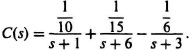
Using partial-fraction expansion, we obtain:
![]()
where

Therefore,
![]()
Taking the inverse Laplace transform of X1(s), we obtain
x1(t) = (0.33 − 0.33e−3t + e−t)U(t)
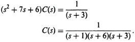
I2.15. Determine the value of c(t) for the following differential equation using the Laplace transform.
![]()
r(t) = e−3tU(t).
SOLUTION: Since
![]()
then

Taking the Laplace transform of this equation, we obtain the following:
![]()
Solving for C(s), we obtain the following:
![]()
Using partial-fraction expansion, we obtain the following:
![]()
where

Therefore,
Taking the inverse Laplace transform of this equation, we obtain
![]()
I2.16. A unit impulse is applied to an element whose transfer function is unknown. If the resulting output is given by
c(t) = 4e−6tU(t)
where U(t) represents a unit step, determine the transfer function of the element.
SOLUTION: Since
![]()
and
R(s) = 1
Therefore,

I2.17. A system is represented by the following differential equation:
![]()
In this differential equation, r(t) represents the input, and c(t) represents the output. Determine the transfer function C(s)/R(s).
SOLUTION: Taking the Laplace transform of this differential equation, we obtain the following:
C(s)(4s2 + 3s + 6) = R(s) + 4R(s)e−s.
Therefore, the transfer function C(s)/R(s) is given by
![]()
I2.18. A system is represented by the following differential equation:
![]()
In this differential equation, r(t) represents the input, and c(t) represents the output. Determine the transfer function C(s)/R(s).
SOLUTION:
Taking the Laplace transform of this differential equation, we obtain the following:
![]()
Simplifying this equation, we obtain the following:
C(s)(s4 + 10s3 + 6s2 + s + 7) = s2R(s) + 3sR(s).
Therefore, the transfer function C(s)/R(s) is given by
![]()
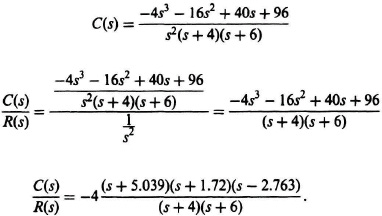
I2.19. We wish to determine the transfer function of an element in a control system. To determine its transfer function, a unit ramp is applied to the input r(t). The output of this element is recorded, and is modelled according to the following equation:
c(t) = (4t − 2e−4t − 2e−6t)U(t).
Determine the transfer function, C(s)/R(s), of this element.
SOLUTION: Since
![]()
and
![]()
simplifying the expression for C(s) results in the following:
I2.20. We wish to determine the transfer function of an element in a control system. Its input, m(t), represents speed, and its output is represented by y(t). To determine its transfer function, a unit step voltage of 1 volt, corresponding to a speed of 1 ft/sec, is applied to the input, m(t). The output of the element is recorded and is modeled according to the following equation:
y(t) = (40 − 8e−5(t−1))U(t − 1)
Determine the transfer function, Y(s)/M(s), of this element. Reduce your answer to its simplest form.
SOLUTION: The Laplace transform of the output y(t) is given by
![]()
Simplifying the expression for Y(s) results in the following:
![]()
Therefore, the transfer function Y(s)/M(s) is given by
![]()
I2.21. The block diagram of a control system is illustrated where R(s) represents the reference input and D(s) represents the disturbance input.
(a) Determine the transfer function C(s)/R(s).
(b) Determine the transfer function C(s)/D(s).
(c) Determine the value of the feedback element H1(s) in order that the disturbance input D(s) has no effect on the output C(s). Assume that R(s) = 0.
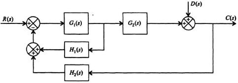
Figure I2.21
SOLUTION: (a) ![]()
(b) ![]()
(c) Setting the numerator of the transfer function C(s)/D(s) = 0, we obtain the following:
1 + G1(s)H1(s) = 0.
Therefore,
![]()
I2.22. The signal-flow graph of a control system is represented by the following, where D(s) represents an external disturbance input into the control system:
(a) Determine the transfer function C(s)/R(s).
(b) Determine the transfer function E(s)/D(s).
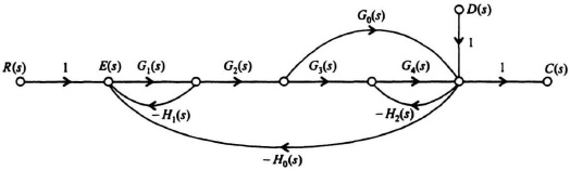
Figure I2.22
![]()
All terms in this transfer function are functions of s.
(b)
![]()
I2.23. Consider the LC ladder network illustrated:

Figure I2.23(I)
The circuit equations representing this LC network are as follows:

(a) Draw the signal-flow graph representing these circuit equations.
(b) Using Mason’s theorem, determine the transfer function, Vout(s)/Vin(s).
SOLUTION: (a)
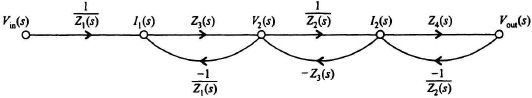
Figure I2.23(II)

I2.24. A feedback control system is represented by the following signal-flow graph:
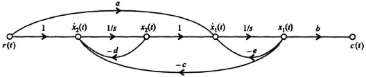
Figure I2.24
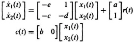
Determine the phase-variable canonical form equations for this feedback control system.
SOLUTION: The differential equations representing this signal-flow graph are given by the following:
![]() 1(t) = −ex1(t) + x2(t) + ar(t)
1(t) = −ex1(t) + x2(t) + ar(t)
![]() 2(t) = −cx1(t) − dx2(t) + r(t).
2(t) = −cx1(t) − dx2(t) + r(t).
The phase-variable canonical equations are given by:
I2.25. Determine the state transition matrix as a sum of an infinite series using Eq. (2.323) for a system whose P matrix is given by:
![]()
Carry out the computation in Eq. (2.323) from k = 0 through k = 2.
SOLUTION:
![]()
I2.26. A system has a companion matrix, P, and an input vector, B, given by the following:
![]()
(a) Determine its state transition matrix using Eq. (2.256).
(b) Solve the state transition equation, Eq. (2.306), for t ≥ 0. Assume that the input is a unit step function, and that the initial state vector is represented by x(0) where
![]()
SOLUTION: (a) From Eq. (2.256):
Φ(t) = ℒ−1{[sI − P]−1}, for t ![]() 0
0
where
![]()
and

Therefore,

(b) From Eq. (2.306):
![]()
where
![]()
![]()
Therefore,
![]()
I2.27. Using the elements presented in Section 2.18 on Operational Amplifiers, develop a flow diagram to simulate the following set of differential equations which represent the model of a system. The outputs from the system are the variables x(t) and y(t).
![]()
Assume the initial conditions are zero.
SOLUTION:
![]()

Figure I2.27