
Equation 1.1 Expected Utility

The chapter begins with a review of two topics that will serve as the foundations of our asset allocation framework: expected utility and estimation error. Asset allocation is then defined as the process of maximizing expected utility while minimizing estimation error and its consequences—a simple yet powerful definition that will guide us through the rest of the book. The chapter concludes with an explicit definition of the modern yet tractable asset allocation framework that is recommended in this book: the maximization of a utility function with not one but three dimensions of client risk preferences while minimizing estimation error and its consequences by only investing in distinct assets and using statistically sound historical estimates as our forecasting foundation.
Key Takeaways:
When deciding whether to invest in an asset, at first glance one might think that the decision is as simple as calculating the expected value of the possible payoffs and investing if the expected payoff is positive. Let's say you are offered the opportunity to invest in a piece of property and the possible outcomes a year from now are a drop of $100,000 and a rise of $150,000, both with a 50% chance of occurring. The expected payoff for the investment is ![]() , so if you only care about expected return, then you would certainly invest.
, so if you only care about expected return, then you would certainly invest.
But are you really prepared to potentially lose $100,000? The answer for many people is no, because $100,000 is a substantial fraction of their assets. If $100,000 represented all of your wealth, you certainly wouldn't risk losing everything. What about an extremely wealthy person? Should they necessarily be enthusiastic about this gamble since the potential loss represents only a small fraction of their wealth? Not if they are very averse to gambling and would much prefer just sitting tight with what they have (“a bird in the hand is worth two in the bush”). When making decisions regarding risky investments one needs to account for (1) how large the potential payoffs are relative to starting wealth; and (2) preferences regarding gambling.
In 1738 Daniel Bernoulli, one of the world's most gifted physicists and mathematicians at the time, posited that rational investors do not choose investments based on expected returns, but rather based on expected utility.1 Utility is exactly what it sounds like: it is a personalized value scale one ascribes to a certain amount of wealth. For example, a very affluent person will not place the same value on an incremental $100 as someone less fortunate. And a professional gambler will not be as afraid of losing some of his wealth as someone who is staunchly opposed to gambling. The concept of utility can therefore account for both effects described in the previous paragraph: potential loss versus total wealth and propensity for gambling. The expected utility (EU) one period later in time is formally defined as
Equation 1.1 Expected Utility
where pi is the probability of outcome i, ![]() is the utility of outcome i, and O is the number of possible outcomes.
is the utility of outcome i, and O is the number of possible outcomes.
Let's now return to our real estate example. Figure 1.1 shows an example utility function for a person with total wealth of $1 million. For the moment, don't worry about the precise shape of the utility function being used; just note that it is a reasonable one for many investors, as will be discussed later in the chapter. Initially the investor's utility is 1 (the utility units are arbitrary and are just an accounting tool2). Given the precise utility function being used and the starting wealth level relative to the potential wealth outcomes, the utility for the positive payoff outcome is 1.5 while the loss outcome has a utility of 0.29, and the expected utility of the investment is 0.9. Since the EU is less than the starting utility of 1, the bet should not be accepted, disagreeing with the decision to invest earlier based purely on expected payoff. If the utility function were a lot less curved downward (imagine more of a straight line at 45 degrees), indicative of an investor with greater propensity to gamble, the expected utility would actually be greater than 1 and the investor would choose to make the investment. Additionally, if the starting wealth of the investor were much less than $1 million, the bet would become less appealing again, as the assumed utility function drops increasingly fast as wealth shrinks, bringing the expected utility well below the starting utility level. Hence, this simple utility construction can indeed account for both gambling propensity as well as the magnitude of the gamble relative to current wealth, as promised.

FIGURE 1.1 Choice Under Uncertainty: Expected Return vs. Expected Utility
The concept of EU is easily extended to a portfolio of assets:
Equation 1.2 Portfolio Expected Utility

where we now first sum over all N assets in the portfolio according to their weights wj, before summing over all O possible outcomes, which ultimately leads to the same formula as Eq. (1.1) except that each outcome is defined at the portfolio level ![]() .
.
How can this help us choose an asset mix for clients? Since utility of wealth is what is important to clients, the goal of wealth management is to maximize the expected utility one period from now.3,4 This is done by starting with Eq. (1.2) and filling in the blanks in four sequential steps: (1) specify the client's utility function; (2) choose assets to include in the portfolio; (3) delineate all possible outcomes and their probability over the next time period; and (4) find the portfolio weights that maximize future EU. These four steps are precisely what is covered in Chapters 2 through 5.
Before moving on, let's take stock of how incredibly insightful this succinct formulation is. The right side of Eq. (1.2) tells us that the advisor's entire mission when building a client's portfolio is to invest in a set of assets that have high probabilities of utility outcomes higher than starting utility (the higher the better) while having as low a probability as possible of outcomes below starting utility (again, the higher utility the better). Just how aggressive we must be in accessing outcomes on the right side of the utility curve and avoiding those on the left is set by the shape of the utility function. For example, utility functions that fall off quickly to the left will require more focus on avoiding the negative outcomes while flatter functions will require less focus on negative outcome avoidance. If we can create an intuitive perspective on the shape of our client's utility function and the return distributions of the assets we invest in, we can build great intuition on the kinds of portfolios the client should have without even running an optimizer. This simple intuition will be a powerful guiding concept as we transition from modern portfolio theory (MPT), which is generally presented without mention of a utility function, to a completely general EU formulation of the problem.
A key proposition of this book is to build client portfolios that have maximal EU as defined by Eq. (1.2). Conceptually, this is a very different approach than the popular mean-variance (M-V) framework, where portfolios are built by maximizing return while minimizing variance, without ever mentioning the client's utility. It is thus imperative to show how deploying the full utility function in the process of building portfolios relates to the MPT framework. It is also time to introduce the most complicated mathematical formula in the book. I promise that the temporary pain will be worth it in the long run and that the reader will not be subjected to any other formulas this complex for the remainder of the book.
The expected utility in our simple real estate example was a function of next period wealth. We will now transition to writing our next period utility outcomes ![]() in Eq. (1.2) in terms of return r rather than wealth, by writing the next period wealth associated with an outcome i as
in Eq. (1.2) in terms of return r rather than wealth, by writing the next period wealth associated with an outcome i as ![]() . Our utility function is now a function of return instead of wealth. The utility function at a particular value of r can then be calculated as a function of successively higher order deviations (linear, squared, cubed, etc.) of r from its mean
. Our utility function is now a function of return instead of wealth. The utility function at a particular value of r can then be calculated as a function of successively higher order deviations (linear, squared, cubed, etc.) of r from its mean ![]() . Here is the formula for writing the utility as a function of the kth order deviation of return from the mean
. Here is the formula for writing the utility as a function of the kth order deviation of return from the mean ![]() :
:
Equation 1.3 Higher Order Expansion of Utility

where ![]() is the kth order derivative of utility evaluated at
is the kth order derivative of utility evaluated at ![]() and
and ![]() , where
, where ![]() . For those familiar with calculus, this is just the Taylor series approximation of our utility function around the point
. For those familiar with calculus, this is just the Taylor series approximation of our utility function around the point ![]() , where the kth order derivative tells us how sensitive a function is to changes in the corresponding kth order change in the underlying variable.
, where the kth order derivative tells us how sensitive a function is to changes in the corresponding kth order change in the underlying variable.
Let's take a look at the first couple of terms. The first term is the zeroth order approximation, where the zeroth order derivative is just the constant ![]() and the zeroth order deviation is just 1, which is just our function value at
and the zeroth order deviation is just 1, which is just our function value at ![]() , a great approximation to U(r) if r is close to
, a great approximation to U(r) if r is close to ![]() . The second term then contains the first order approximation, which says that as r deviates from μ, the function roughly changes by the amount of the first derivative multiplied by linear changes in return relative to the mean
. The second term then contains the first order approximation, which says that as r deviates from μ, the function roughly changes by the amount of the first derivative multiplied by linear changes in return relative to the mean ![]() . Each successive term just brings in higher order derivatives and deviations to make additional adjustments to the series approximation of the full function.
. Each successive term just brings in higher order derivatives and deviations to make additional adjustments to the series approximation of the full function.
The benefit of writing a function in terms of higher order deviations is that at some point the higher order terms become very small relative to the first few terms and can be ignored, which can often help simplify the problem at hand. This approximation should look familiar to anyone who has studied the sensitivity of bond prices to interest rates. A bond's price as a function of interest rates can be approximated via Eq. (1.3) by substituting bond price for utility and setting ![]() . Then the first order bond price equals the current price (zeroth order term) plus the first derivative of bond price with respect to rates (bond duration) multiplied by the change in rates. For larger moves in interest rates one must then account for second order effects, which is just the second derivative of bond price with respect to rates (bond convexity) multiplied by squared changes in interest rates.
. Then the first order bond price equals the current price (zeroth order term) plus the first derivative of bond price with respect to rates (bond duration) multiplied by the change in rates. For larger moves in interest rates one must then account for second order effects, which is just the second derivative of bond price with respect to rates (bond convexity) multiplied by squared changes in interest rates.
It is now time for the punchline of this section. Inserting Eq. (1.3) into Eq. (1.2), the expected utility for a portfolio of assets can be written as:
Equation 1.4 Utility as a Function of Moments
an infinite series we are only showing the first four5 terms of. ![]() is the kth order derivative of utility evaluated at
is the kth order derivative of utility evaluated at ![]() ,
, ![]() is the portfolio expected return,
is the portfolio expected return, ![]() is the portfolio expected volatility,
is the portfolio expected volatility, ![]() is the portfolio expected skew, and
is the portfolio expected skew, and ![]() is the portfolio expected kurtosis. In statistics, these last four quantities are also known as the first, second, third, and fourth “moments” of the portfolio's distribution of returns, since the kth moment is defined as the expected value of
is the portfolio expected kurtosis. In statistics, these last four quantities are also known as the first, second, third, and fourth “moments” of the portfolio's distribution of returns, since the kth moment is defined as the expected value of ![]() .
.
Any return distribution can be completely characterized by its full set of moments, as each moment provides incrementally distinct information about the shape of the return distribution, almost as if each moment is like a partial fingerprint of the distribution. The first moment describes the location of the center of the distribution; the second moment describes the width of the distribution; the third and fourth moments characterize how asymmetric and fat-tailed the distribution is, respectively. It is expected that the reader is familiar with the first two moments but not the next two, which are reviewed in depth in the following section.
Upon solving for the expected value of the series approximation to a utility function, the kth order deviation turned into the kth order moment, an exciting turn of events. Equation (1.4) demonstrates that the maximization of portfolio EU, the core goal for any wealth manager, amounts to maximizing over an infinite set of moments. A typical utility function we will consider will have a positive first derivative and negative second derivative (much more on this later). Therefore, when typically maximizing EU, we are searching for maximal portfolio return and minimal portfolio variance while also maximizing an infinite set of other portfolio return moments whose derivatives (and resulting signs in Eq. (1.4)) are to be determined. MPT is now clearly an approximation to the full EU maximization process we really want to consider! The M-V optimization solution is what is known as a “second order” approximation to the full solution, since it only considers the first two terms of the problem.
In the following section we review the conditions under which we should be concerned with higher order terms missing in M-V, and from there we show precisely how we are going to approach the problem without making a second order approximation (completely avoiding what is formally known as “approximation error”) (Adler & Kritzman, 2007; Grinold, 1999). We are in good company here: Markowitz himself has said that if mean-variance is not applicable, then the appropriate solution is the maximization of the full utility function (Markowitz, 2010).
For all readers who have made it to this point, thank you for bearing with me through the most mathematical part of the book. At this point you no longer have to worry about Eq. (1.3), which was solely introduced to derive Eq. (1.4), the key result of the section and one that will be used throughout the book. I encourage any readers not fully comfortable with Eq. (1.4) to go back and reread this section, noting that Eq. (1.3) is a mathematical complexity that can be glossed over as long as Eq. (1.4) is fully baked into your psyche.
It was just shown that MPT is a second order approximation to the full problem we ideally want to solve. A natural question now is whether the chopped off third and higher terms that MPT is missing is a critical deficiency. If it is, then the maximization of the full utility function becomes a necessity. But it is quite hard to generalize the answer to the question, since it is highly dependent on the utility function of the client, and the expected moments of the assets being deployed; and we will not have those answers for a few more chapters still. Even then the answers will vary for every single client and portfolio, and will even change over time as capital markets evolve.
At this stage, though, we are focused on motivating a compelling asset allocation framework; hence the key question we must address is whether there is a chance for higher order terms to come into play. To this end, it should be noted that higher order terms do not exist in Eq. (1.4) unless two criteria are met: (1) portfolio return distributions have third or higher moments; and (2) our utility function has a preference regarding those higher moments (i.e. it has non-zero third order derivatives or higher). By studying higher moment properties of some typical investable assets and higher order preferences embedded in typical utility functions, you will see that both conditions are generally met, and higher order terms should be accounted for in the process.
Before we tackle the first condition by investigating whether typical assets have higher moment characteristics, let's first build up our general understanding of the third and fourth moments—skew and kurtosis, respectively. The easiest way to think about higher moments is to start from the most common distribution in mother nature, the normal distribution.6 The important thing to know about the normal distribution is that it is symmetric about the mean ![]() , and its tails are not too skinny and are not too fat
, and its tails are not too skinny and are not too fat ![]() . Figure 1.2 shows a normal distribution of monthly returns, with mean of 1% and volatility of 2%; this will serve as our baseline distribution, to which we will now add higher moments.
. Figure 1.2 shows a normal distribution of monthly returns, with mean of 1% and volatility of 2%; this will serve as our baseline distribution, to which we will now add higher moments.
The easiest way to intuit the effect of negative skew is to imagine a tall tree, firmly rooted in the ground and standing up perfectly straight. If one were to try to pull the tree out of the ground by tying a rope to the top of the tree and pulling to the right, the top of the tree would begin to move right and the roots on the left side of the tree would start to come out of the ground while the roots on the right side would get compressed deeper into the ground. This is why in Figure 1.2 the peak of the distribution with skew of −0.5 is slightly right of the normal distribution peak while the left tail is now raised a bit and the right tail is cut off slightly. Hence, a negatively skewed distribution has a higher frequency of extremely bad events than a normal distribution while the number of events just above the mean goes up and the number of extreme positive events goes down. Positive skew is the exact opposite of the situation just described (a tree now being pulled out to the left): positive skew distributions have a higher frequency of extremely favorable events than a normal distribution while the number of events just below the mean goes up and the number of extreme negative events goes down.

FIGURE 1.2 Skew and Kurtosis Effects on a Normal Distribution
Kurtosis, on the other hand, is a symmetrical effect. The way I intuit kurtosis above 3 is to imagine wrapping my hand around the base of a normal distribution and squeezing, which forces some of the middle of the distribution out into the tails (through the bottom of my fist) and some of the middle of the distribution up (through the top of my fist). Therefore, a kurtosis above 3 implies, relative to a normal distribution, more events in both tails, more events at the very center of the distribution, and less middle-of-the-road events. Decreasing kurtosis from 3 then has the exact opposite effect: fewer events will happen in the tails and in the very center of the distribution relative to a normal distribution, in exchange for more mediocre positive and negative outcomes. Figure 1.2 shows a distribution with a kurtosis of 6, where you clearly see an increase in the number of events in the middle of the distribution at the expense of fewer middle-of-the-road deviations from the mean; and with a bit more strain you can see the increased number of tail events (the signature “fat tails” of high kurtosis distributions). This moment may remind you of the second moment (volatility), due to its symmetry. But note that volatility controls the width of the distribution everywhere while kurtosis has different effects on the width of the distribution at the top, middle, and bottom: when we raised kurtosis from 3 to 6, the width of the distribution widened at the top, shrank in the middle, and widened at the very bottom.
Now that we are familiar with skew and kurtosis, let's return to the first point we would like to prove. To simplify things, we will not be looking at portfolio higher moments; instead, we will look at the higher moments of the underlying assets. While this is not the precise condition we are out to prove, the existence of asset-level higher moments should certainly put us on alert for the existence of portfolio-level higher moments.7
Figure 1.3 plots the third and fourth moments for some common publicly traded assets, where we clearly see that most assets indeed have higher moments associated with their distributions; therefore QED on our first point.8,9 But let's pause and make sure we understand the results. For instance, why do 3 Month Treasuries have such extreme positive skew? And why do equities show up on the opposite side of the skew spectrum?
Given our understanding of how positively skewed distributions are shaped, it is hopefully rather intuitive why short-term US Treasuries are positively skewed: they have very limited left tail risk given their minimal duration10 or credit risk while simultaneously offering the potential for some outsized moves to the upside as a flight-to-quality play during times of stress. At the other extreme is US equities, an asset class that intuitively leaves the investor susceptible to negative skew via extreme liquidity events like the Great Recession. Figure 1.3 also shows a of couple long/short alternative risk premia assets: the Fama-French value factor (F-F HML) and the Fama-French robustness factor (F-F RMW), along with a strategy that is split 50/50 between these two factors. As you can see, these market-neutral equity strategies have the ability to introduce both positive skew and kurtosis relative to their underlying equity universe.

FIGURE 1.3 Skew and Kurtosis of Common Modern Assets (Historical Data from 1972 to 2018)10
In Chapter 3 we will spend time reviewing the landscape of risk premia, and in that process we will build a generalized understanding of how skew is introduced to investment strategies. As you will see then, I believe that one of the key innovations within investment products over the next few decades will be increasingly surgical vehicles for accessing higher moments (via alternative risk premia), a key motivation for the inclusion of higher moments in our asset allocation framework.
Let's now move to the second minimum condition to care about higher moments: clients must have preferences when it comes to higher moments; that is, a client's utility function must be sensitive to the third moment or higher. For now we will analyze this question generally, as we have still not formally introduced the utility function we will be deploying.
Empirical work on the higher moment capital asset pricing model (CAPM) (Kraus & Litzenberger, 1976) was one of the first lines of research that showed us that investors prefer positive skew by virtue of requiring compensation for negative skew. Just as the CAPM showed us that expected returns increase with volatility (investors demand higher returns to hold more volatile assets), the higher moment extension of CAPM shows us that expected returns increase as skew becomes increasingly negative (investors demand higher returns to hold more negatively skewed assets).
It has also been shown that if our utility function is such that the investor always prefers more wealth to less (utility is always increasing with wealth/return), and that the benefit of extra wealth fades as wealth increases (the slope of your utility function gets less and less positive with wealth/return), we have preferences for positive skew and negative excess kurtosis (Scott & Horvath, 1980).11 And the result is even more powerful than that: these assumptions allow you to draw the conclusion that an investor should prefer all odd moments to be high and all even moments to be low! We have arrived at a key result very rigorously, and at the same time the even versus odd preference seems to be rather intuitive for a rational investor. As reviewed earlier in the chapter, a rational investor wants to earn money while avoiding the risk of ruin and without gambling beyond their preferred limits, which is just saying that a rational investor prefers high returns while avoiding drawdowns and dispersion. Hence, an optimal portfolio for a rational investor would have large returns (large first moment), minimal drawdowns (large third moment and small fourth moment), and minimal dispersion (low second moment), showcasing a clear preference for odd moments and an aversion to even moments. But let's pause our discussion on higher moment preferences until we have introduced the precise utility function we will deploy. Hopefully we have motivated the fact that under a simple set of assumptions about client utility (which you will see shortly often applies to real-world utility functions), individuals will have clear preferences toward higher moments and we don't want to ignore these preferences.
At this point we have shown that many common assets have statistically significant higher moments, and that clients will often have well-defined preferences to higher moments, validating that we should indeed be wary that higher moments could play a role in building client portfolios. But we have not yet discussed the magnitudes of the higher order utility derivatives or portfolio moments, which determine the size of the higher order terms relative to the first two terms in Eq. (1.4), and ultimately inform whether these terms play a meaningful role in the EU maximization problem. As seen firsthand in the portfolios we create in Chapter 5, today's most common asset classes and their particular expected returns often lead to an EU solution that is predominantly a simple tradeoff between return and volatility. Hence, despite the fact that utility functions generally have higher moment preferences and assets are typically non-normal, the higher order terms can often have minimal effects. Unfortunately, it is impossible to know this, a priori, for a given client utility and investment universe. The only way to know for sure is to deploy the full utility function and analyze the results, which is clearly a reasonable prerequisite given the preceding presentation. The expected moments will also change in time as market environments ebb and flow. If, all of a sudden, return forecasts are cut across the board while the utility function and assets deployed are unchanged, higher order terms that were once inconsequential could potentially become relevant—a complete unknown until we are actually there.
As you will see in Chapter 3, there appears to be a natural evolution in the asset management industry toward investment products that are more focused on the exploitation of higher moments, where we would expect an increase in the number of assets whose higher moments can indeed influence the asset allocation decision. We have already seen the first generation of this trend make its way to the retail space in the form of style premia and option strategies, both born in the land of hedge funds, where higher moments are a key input to any asset allocation process (Cremers, Kritzman, & Page, 2004). And given the ease with which we can run optimizers over the full utility function these days, there is little computational hurdle to deploying a framework that avoids lower-order approximations.
The most pressing issue with MPT in today's markets and for a typical retail client is not the missing higher order terms in Eq. (1.4). Rather, it is the more practical question of how to find the second derivative of utility,12 which plays a critical role in setting the precise portfolios that MPT recommends for clients. It turns out that once behavioral risk preferences are accounted for (introduced in the next section), a singular measure of risk preference is insufficient.
Let's assume that markets are fully described by the first two moments. The second derivative in Eq. (1.4) is a measure of a client's aversion to volatility (with a negative sign pulled out in front of it), which many practitioners intuit for their clients as they get to know them personally or through some form of risk tolerance questionnaire. Advisors then assign a client to one of four or five volatility-targeted portfolios on the M-V efficient frontier (clients with lower perceived risk aversion will be assigned a portfolio with higher volatility, and vice versa). I have no issue with the fact that clients are generally only binned into four or five buckets, since estimation error often prevents much more granular assignments, as reviewed in Chapter 5. Nor, at the moment, am I flagging the methods of measuring preferences just described (although I do believe the more mathematical system laid out in Chapter 2 for measuring risk preferences is superior to the standard qualitative questionnaire, and certainly better than an intuitive read of a client). I am also not flagging the sole use of a second order approximation, where clients are binned solely by their volatility, since for this exercise I am assuming markets are fully described by the first two moments. Rather, I have issue with the second derivative being assessed as a singular number.
In the following section we will introduce our modern utility function, which has three parameters, including the traditional (rational) risk aversion parameter, along with two behavioral (irrational) parameters. Then, in Chapter 2, we will show that to account for financial goals we must moderate the three preferences. A critical feature of our goals moderation system is that each parameter must be moderated independently; therefore we cannot simply lump them into a single volatility aversion. Indeed, if our client had no financial goals, we could just measure the full utility function and fit it for a constant second derivative, avoiding the specification of a utility function that requires careful delineation between three different preference types. The inclusion of financial goals in the presence of irrational risk preferences requires us to fully divorce ourselves from MPT. If this is confusing right now, don't despair; Chapters 2 and 5 will make it clearer.
With that said, even in the absence of financial goals, I believe it is wise still to deploy the fully utility function introduced in the following section. Its three distinct risk preference parameters provide a rich amount of detail that an advisor can work through with his or her client. In addition to providing a very accurate assessment of the client's utility function and all its derivatives, this modern tool also allows both advisor and client to understand quickly the client's risk preferences in a powerful and intuitive framework. So, even in the case of no financial goals, one can gain a lot of intuition around the subtle behaviors that create utility curvature by measuring our three risk preferences and painting a full picture behind the singular volatility aversion parameter.
Of course, in the cases where higher moments indeed matter, the full utility function will indeed provide additional higher moment preference information that is relevant.
As you will see starting in Chapter 2 (and starkly punctuated in our discussions in Chapter 5), by combining modern perspectives on utility functions with the full utility optimization routine, we will generate a very nuanced but intuitive and accurate prescription for matching client preferences and goals to an appropriate portfolio.
It is now time to introduce the utility function we will deploy for the remainder of the book. Utility functions are completely unfamiliar to us in our everyday life, so it is imperative that we connect this mathematical representation of risk preferences to clearly identifiable and intuitive behaviors. To this end, I begin with a review of the simplest utility function that may satisfy a client's preferences, and then iteratively introduce two modifications to that function to account for two additional types of risk preferences. The section concludes with the formal definition of a generalized utility function, which we will use for the remainder of the book to succinctly capture all three “dimensions” of risk preferences that are key for building portfolios.13
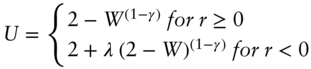
The traditional (AKA neoclassical) utility function used in economics for rational investors is the power utility, with its single parameter risk aversion ![]() :
:
Equation 1.5 Power Utility
where W is the single period wealth change ![]() , r is the single period portfolio return (we drop the “port” subscript from here on since for the remainder of the book we will only be considering utility outcomes for a portfolio of assets), and
, r is the single period portfolio return (we drop the “port” subscript from here on since for the remainder of the book we will only be considering utility outcomes for a portfolio of assets), and ![]() is parameterized between 1.5 and 12 (as detailed in Chapter 2).14 Power utility is plotted as a function of r in Figure 1.4 with
is parameterized between 1.5 and 12 (as detailed in Chapter 2).14 Power utility is plotted as a function of r in Figure 1.4 with ![]() and is precisely the same utility function plotted in Figure 1.1.
and is precisely the same utility function plotted in Figure 1.1.

FIGURE 1.4 Graphical Representation of Utility Functions ( ,
,  )
)
This function fulfills the two key intuitive attributes we require from our baseline utility function, which happen to be the exact same attributes required earlier to be able to say a client always prefers high odd moments and low even moments:
It is interesting to note that this function, which was the darling of economists for most of the twentieth century, is well approximated by Markowitz's simple mean-variance framework for low levels of risk aversion or highly normal return distributions (Cremers, Kritzman, & Page, 2004). This key fact, combined with the solvability of M-V on the earliest of modern computers, explains why mean-variance has been so dominant in the world of asset allocation. But this function, by virtue of being well represented by the MPT solution, roughly has no opinion on skew or higher moments. It is probably safe to assume that no rational investor, even if their risk aversion is on the low end of the spectrum, is agnostic to even moderate levels of negative skew; so it is hard to accept power utility as our core utility function. As an example, look at both principal and agent responses to the Great Recession: many clients and advisors need portfolios that avoid large exposure to negative skew to be able to keep them invested in a long-term plan.
A kinked utility function, with its two parameters, risk aversion ![]() and loss aversion
and loss aversion ![]() (parameterized here from 1.5 to 12 and 1 to 3, as detailed in Chapter 2), satisfies our two simple criteria while additionally having the practical third moment sensitivity we require:15
(parameterized here from 1.5 to 12 and 1 to 3, as detailed in Chapter 2), satisfies our two simple criteria while additionally having the practical third moment sensitivity we require:15
Equation 1.6 Kinked Utility

As you can see, kinked utility is the same as the power utility when returns are positive; but when returns are negative, the utility drops at a rate ![]() times as fast, giving us clear preference toward positive skew (and away from negative skew) when
times as fast, giving us clear preference toward positive skew (and away from negative skew) when ![]() is greater than 1 (when
is greater than 1 (when ![]() equals 1 this function is the same as Eq. (1.5)). Figure 1.4 shows the kinked utility with risk aversion
equals 1 this function is the same as Eq. (1.5)). Figure 1.4 shows the kinked utility with risk aversion ![]() and loss aversion
and loss aversion ![]() , where you can clearly see the kinked utility drop faster than the power utility with the same risk aversion in the loss domain, since
, where you can clearly see the kinked utility drop faster than the power utility with the same risk aversion in the loss domain, since ![]() . But admittedly, at this point we are just postulating this specific form for an asymmetric utility function. Can we justify the kinked utility function with more than just our intuition on investor preferences to negative skew?
. But admittedly, at this point we are just postulating this specific form for an asymmetric utility function. Can we justify the kinked utility function with more than just our intuition on investor preferences to negative skew?
Enter prospect theory (PT) (Kahneman & Taversky, 1979), a key advance in our understanding of real-world risk preferences from the discipline of behavioral economics, where psychology meets economics. This descriptive theory of real human behavior introduces two new “irrational” features of decision-making under uncertainty to the “rational” theory encapsulated by our power utility function.
The first is “loss aversion,” where an investor feels the emotional drain of losses disproportionately more than they feel the emotional benefit of gains. The more loss aversion one has, the more unwilling they will be to play a game with very favorable terms if there is the possibility of losing even a small amount of money. For example, someone with strong loss aversion would not flip a coin where they stood to win $100 on heads and lose $20 on tails, a very favorable game that any robot (AKA neoclassical investor) would happily play.
The second PT feature is “reflection,” where investors are risk averse only when it comes to gains and are risk seeking when it comes to losses. Unlike the power utility function investor, who always prefers their current situation to a 50/50 chance of winning or losing the same amount (since the utility second derivative is negative), an investor with reflection will actually favor the aforementioned 50/50 gamble if they are in a losing situation. For example, a client with reflection who owns a stock with a paper loss of 20%, where from here the stock can either get back to even or drop another 20%, would choose to roll the dice, whereas a client who is risk averse across both loss and gain domains would not risk the possibility of further loss. Another way to think of reflection is that it represents the joint emotions of “hoping to avoid losses” (risk-seeking in the loss domain) while being “afraid of missing out on gains” (risk-averse in the gain domain), which precisely agrees with the well-known phenomenon where amateur traders cut winners too quickly and hold onto losers too long.
Both PT effects require us to shift from thinking of utility in terms of wealth to thinking in terms of gains and losses, since both new preference features require a clear distinction between losses and gains.16 For a gentle yet detailed overview of PT, see Levy's review (Levy, 1992).17 But for a quick and intuitive overview, a fantastic description of PT was provided to me by my father, who, upon completing the risk preference diagnostics I review in Chapter 2, turned to me and said, “I don't like risk, but I like to win.” This statement validates the risk profile I have developed for my father over 40 years of getting to know him. It also perfectly represents the average PT client, who “doesn't like risk” (which I interpret as including both risk and loss aversion) but “likes to win” (which I interpret as being risk-seeking in the loss domain in an effort to avoid realizing a loss). And yes, my father's risk preference questionnaire results clearly flagged him for both loss aversion and reflection.
The kinked utility function already introduced indeed addresses prospect theory's loss aversion effect precisely; therefore we have grounded that iteration of our utility function on solid behavioral research grounds. But what about reflection? The S-shaped utility function will do the trick. To continue down our intuitive path connecting power to kinked to S-shaped utility as we introduce new dimensions of risk preferences, I again stitch together two power functions across the gain and loss domains, with some simplified parameterization to construct the S-shaped utility:18
Equation 1.7 S-Shaped Utility
This function has the same two parameters as the kinked function, risk aversion ![]() and loss aversion
and loss aversion ![]() , but now in the domain of losses our utility function actually curves up rather than going down, resembling the shape of the letter “S.” Figure 1.4 shows the S-shaped utility function with
, but now in the domain of losses our utility function actually curves up rather than going down, resembling the shape of the letter “S.” Figure 1.4 shows the S-shaped utility function with ![]() and
and ![]() . One can clearly see the function fall off faster than the power function as you first enter the loss domain due to the loss aversion of 3; but as you proceed further into the loss domain the function curves up due to the reflection embodied in the S-shaped function, which implies a preference for risk on the downside. Note that we have assumed that the reflection effect is symmetric (i.e. we have the same
. One can clearly see the function fall off faster than the power function as you first enter the loss domain due to the loss aversion of 3; but as you proceed further into the loss domain the function curves up due to the reflection embodied in the S-shaped function, which implies a preference for risk on the downside. Note that we have assumed that the reflection effect is symmetric (i.e. we have the same ![]() in both gain and loss domains). You can indeed make this S-shaped function more complicated by assuming asymmetric curvature in the gain and loss domains, but in an effort to keep the story simple we will assume the same curvature parameter
in both gain and loss domains). You can indeed make this S-shaped function more complicated by assuming asymmetric curvature in the gain and loss domains, but in an effort to keep the story simple we will assume the same curvature parameter ![]() in both domains. While studies have shown that population averages of loss and gain domain curvature are very symmetric, there can indeed be significant departure from symmetry at the individual level (Kahneman & Taversky, 1979; Abdellaoui, Bleichrodt, & Paraschiv, 2007), a feature an advisor may wish to capture if it doesn't add too much burden to their measurement process and presentation to clients.
in both domains. While studies have shown that population averages of loss and gain domain curvature are very symmetric, there can indeed be significant departure from symmetry at the individual level (Kahneman & Taversky, 1979; Abdellaoui, Bleichrodt, & Paraschiv, 2007), a feature an advisor may wish to capture if it doesn't add too much burden to their measurement process and presentation to clients.
In order to systematically capture all three client risk preferences we have reviewed thus far via a single utility function, we define a generalized utility function that can fluidly evolve based on all three dimensions of risk preferences:19
Equation 1.8 Three-Dimensional Risk Profile Utility Function

This function has both risk aversion ![]() and loss aversion
and loss aversion ![]() , but now there is one additional parameter
, but now there is one additional parameter ![]() , which takes on the value of 1 when reflection should be expressed, and 0 when there is no reflection. Equation (1.8) is our final utility function, which collapses to Eq. (1.7) when
, which takes on the value of 1 when reflection should be expressed, and 0 when there is no reflection. Equation (1.8) is our final utility function, which collapses to Eq. (1.7) when ![]() , collapses to Eq. (1.6) when
, collapses to Eq. (1.6) when ![]() , and collapses to Eq. (1.5) when
, and collapses to Eq. (1.5) when ![]() and
and ![]() . From here on out we will solely reference our three-dimensional risk profile utility defined in Eq. (1.8), as it fully encapsulates all three dimensions (
. From here on out we will solely reference our three-dimensional risk profile utility defined in Eq. (1.8), as it fully encapsulates all three dimensions (![]() ,
, ![]() , and
, and ![]() ) of a modern client risk profile.
) of a modern client risk profile.
Earlier in the chapter we argued generally that client preference would be for higher skew and lower kurtosis. The power and kinked utility functions indeed preserve that general preference for odd moments and aversion to even moments, since their first derivative is always positive (utility always increases with return) and their second derivative is always negative (utility is always concave). However, with the introduction of reflection we must reassess that set of preferences. For our three-dimensional risk profile utility when ![]() , these preferences now depend on all three parameter choices (Cremers, Kritzman, & Page, 2004), as the second derivative is no longer negative for all returns, and preference moments will be determined by the competing forces of risk aversion, loss aversion, and reflection. The bottom line is that moment preferences depend on the precise parameters of our three-dimensional risk profile utility function, where we know those preferences only with certainty when
, these preferences now depend on all three parameter choices (Cremers, Kritzman, & Page, 2004), as the second derivative is no longer negative for all returns, and preference moments will be determined by the competing forces of risk aversion, loss aversion, and reflection. The bottom line is that moment preferences depend on the precise parameters of our three-dimensional risk profile utility function, where we know those preferences only with certainty when ![]() . With that said, we do not have to harp on the topic of moment preferences any longer, as the core proposition of this book is to maximize the expected utility, which automatically accounts for all higher moment preferences; hence advisors need not dissect individual moment preferences for their clients. Hopefully, though, the discussion of moment preferences has added some interesting color around the nuances of the utility function we will be deploying.
. With that said, we do not have to harp on the topic of moment preferences any longer, as the core proposition of this book is to maximize the expected utility, which automatically accounts for all higher moment preferences; hence advisors need not dissect individual moment preferences for their clients. Hopefully, though, the discussion of moment preferences has added some interesting color around the nuances of the utility function we will be deploying.
In Chapter 2, I will review how to set our utility function parameters ![]() ,
, ![]() , and
, and ![]() . But before we move away from our discussion on maximizing utility, let's discuss how we will actually go about maximizing the full utility function, and not just optimizing a lower order approximation.
. But before we move away from our discussion on maximizing utility, let's discuss how we will actually go about maximizing the full utility function, and not just optimizing a lower order approximation.
Clearly the real asset allocation problem we want to solve is the maximization of the full utility function. But what exactly does that look like when the rubber meets the road? In the classic MPT solution we input expected returns, variances, and covariances into an optimizer to find portfolios that maximize expected returns while minimizing expected variance, which can conveniently be plotted as a 2-D efficient frontier. But what are the inputs into the optimizer when maximizing EU? And what outputs are we plotting in the case of the full utility, if there are no moments to speak of?
Equation (1.2) is the precise definition of what we will now be maximizing: expected utility over all possible outcomes. But how exactly do you define an outcome in the maximization of EU across a set of assets? An outcome is simply one possible joint outcome of all assets (i.e. the returns for all assets during the same period). From here on we will use a monthly return period to define an outcome, since this is roughly the period over which client-concerning drawdowns can generally occur. Hence, we formally define a single outcome as the returns for all our assets during a single month. We can then calculate the portfolio utility ![]() for each outcome i, defined by an exhaustive set of monthly joint return outcomes (AKA the joint return distribution) and our client's utility function, which is a function of the portfolio asset allocation (what we are solving for, AKA the decision variable). Once we set the probability
for each outcome i, defined by an exhaustive set of monthly joint return outcomes (AKA the joint return distribution) and our client's utility function, which is a function of the portfolio asset allocation (what we are solving for, AKA the decision variable). Once we set the probability ![]() for each outcome, we can run an optimizer that will find the weights of the assets in the portfolio that maximize the expected value of utility over all outcomes.
for each outcome, we can run an optimizer that will find the weights of the assets in the portfolio that maximize the expected value of utility over all outcomes.
But how do we create a complete list of possible outcomes and their probabilities? To facilitate generation of future outcomes we will utilize the entire set of historical outcomes. The returns for our assets during an individual month in history will represent a single outcome, where the full historical set of months will represent all possible outcomes, and we will assume equal-weighted probability for each outcome. Chapter 4 is fully dedicated to validating our use of historical joint returns as a starting point for our outcome forecasts, where we will also provide techniques for manipulating the outcomes to account for personalized market forecasts, taxes, and other key adjustments.
Returns-based optimization has been around for a long time, and while it may sound complex or esoteric, it is really neither. I personally think this concept is rather simple once it is grasped. It connects in a very natural way the investment portfolio to the actual thing we care about, our client's utility. Just think about how intuitive our real estate example was at the beginning of the chapter. There was no discussion of moments, just a couple of possible outcomes and a utility function that helped make our choice. I also think it's beautifully elegant in the way it collapses away all discussions of moments by calculating the ![]() , which accounts for all possible asset and cross-asset information. It never ceases to amaze me that every subtle relationship between assets, whether linear (covariance) or non-linear (coskewness, cokurtosis, etc.), is captured by the sequential list of joint return outcomes.
, which accounts for all possible asset and cross-asset information. It never ceases to amaze me that every subtle relationship between assets, whether linear (covariance) or non-linear (coskewness, cokurtosis, etc.), is captured by the sequential list of joint return outcomes.
Before we leave this high-level discussion of our optimization framework, I want to point out that you will not see any efficient frontiers in this book. As alluded to earlier when discussing client risk preference measurements, a key benefit of a mean-variance efficient frontier is that one can bin clients into different sections of the frontier based on volatility targets, which helps avoid a more formal/mathematical description of the client's aversion to volatility. But in our approach, we begin by precisely diagnosing the client's preferences as defined by our three utility parameters and then run the optimizer for the singular utility function defined by the client's personal parameters, producing just a single portfolio that is appropriate for our client. This approach completely avoids having to create all possible optimal portfolios and then slotting a client into one of them; hence the lack of need for an efficient frontier. This may sound pedantic, but the distinction is rather important regarding the accuracy of our process for defining client preferences. As you will see, in a framework characterized by well-defined and intuitive risk preference parameters, we will have more reason to plot all possible portfolios as a function of the three utility parameters than to plot them as a function of one or more moments.
Anyone who has attempted to run a quantitative asset allocation process that deploys an optimizer is very aware of how sensitive the results can be to the assumptions. In the case of mean-variance optimization, it is well known that relatively small changes in return expectations can cause dramatic changes in the recommended asset allocation of the optimizer. Figure 1.5 shows the recommended asset allocation of a mean-variance optimizer for two assets, US large cap equities and US small cap equities, as a function of the expected annual return for US large caps that is fed into the optimizer.20 As you can see, only a 2% shift in return expectation flips the recommended portfolio from all small cap to all large cap. This kind of sensitivity is an incredibly large hurdle for widespread adoption of optimized asset allocation frameworks, since it prevents users from gaining confidence that the optimization process is a worthwhile exercise.
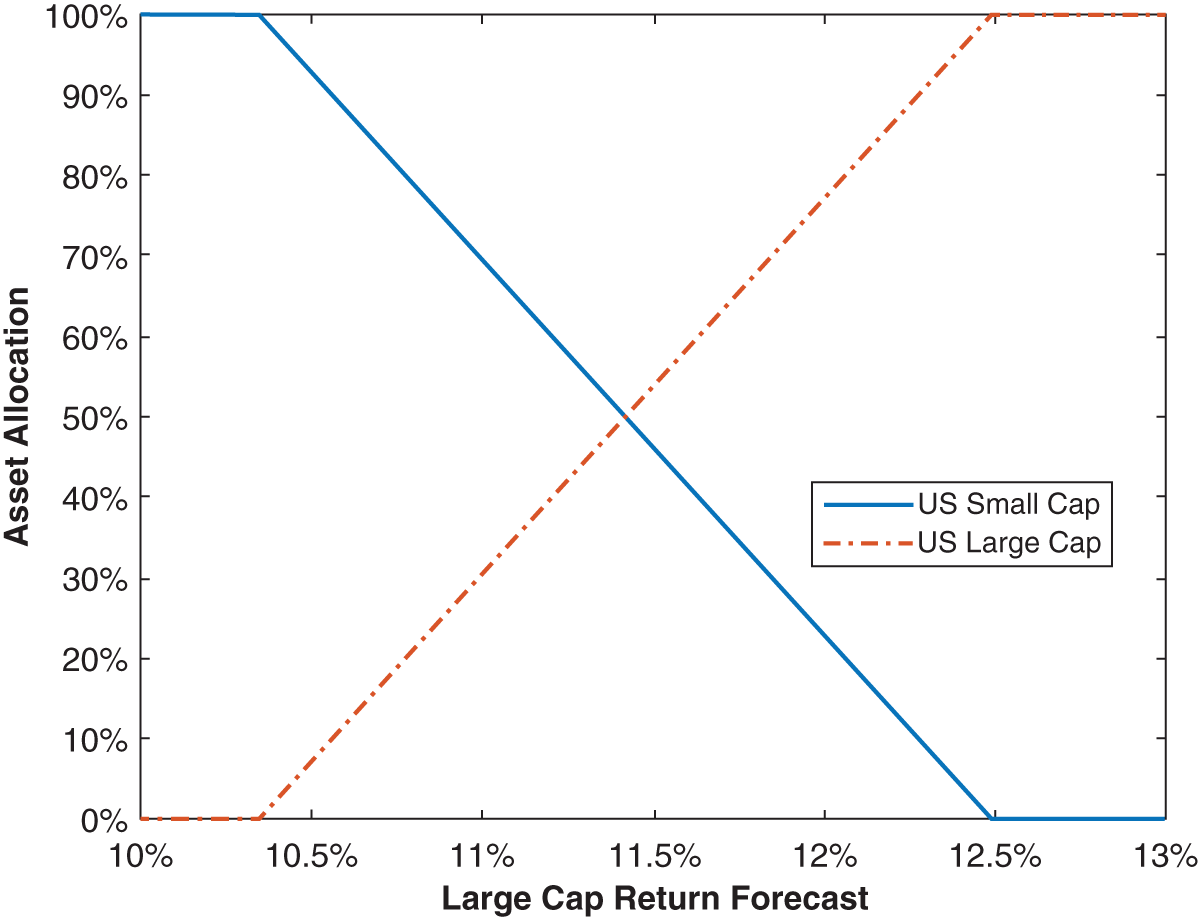
FIGURE 1.5 Allocation Sensitivity to Forecasts
Can we assign blame here? Is the optimizer an overly sensitive tool that needs to be treated with great care or do users of optimizers need to be world-class forecasters who can stand behind the resulting optimizer prescription regardless of its sensitivity? The answer is both. Ideally we would have forecasts that are 100% accurate, which have zero error bars around them (i.e. they have zero estimation error), and we can let the optimizer loose with full confidence. But this is never the case and we additionally want our optimizer to not be overly sensitive to the error bars on our inputs. Thus there are two topics that must be tackled by advisors: how to minimize estimation error and how to minimize the sensitivity to estimation error. Let's begin with estimation error itself and how to minimize it.
The ideal situation for anyone trying to forecast the long-term behavior of a random process, such as the joint monthly return stream for a universe of investable assets over long horizons (10+ years) as we are doing here, is to know that the distribution of the process we have seen in the past is precisely the distribution we will see in the future.21 In this instance we know what statisticians call the “true” distribution, and everything we can know about the process is contained in its historical distribution. In this case one can just use the measured distribution as their forecast and they would have a perfect estimate (zero estimation error).
Using historical data for your forecast in this manner is known as non-parametric estimation, since one doesn't specify any functional forms or parameters during the estimation process, and you have completely avoided any approximation error (similar to what we are doing by using the full utility function instead of M-V). Given the lack of any function or parameter specification, this technique also qualifies as the simplest of all estimation techniques. Therefore, non-parametric estimation from a true distribution is simultaneously the most accurate and the simplest forecasting technique possible. The rub here is the assumption that we are looking at the true distribution. How do we know we have measured the true return distribution of the asset and not just a moderately representative sample of the true distribution?
We now introduce the two key concepts that help answer this question: sample size and stationarity. The precise measurements of these two metrics will be the primary focus of Chapter 4, but for now we will take a moment to lay the groundwork for where we are headed. Let's take a look at sample size first.
Sample size is the number of observations that are in the measured return distribution. If the number of observations is small, there is no way the true distribution of the asset can be measured. On the flipside, if the number of measurements is large enough, we actually have a shot at reconstructing the true distribution. An extreme example brings this point home. If I told you I measured the Standard & Poor's (S&P) 500 return for two months and was going to assume that all months for the next 10 years behaved similar to those two measured months, you would call me crazy, and rightfully so, given that my sample size is comically small. In Chapter 4 we will introduce precise criteria that inform us whether our sample size is sufficient to create a reasonable measure of the true distribution.
When we know for sure that there are not enough observations to accurately reconstruct the true distribution (i.e. our sample size is limited for one reason or another), there are a number of interesting techniques that try to assist the forecaster by introducing structure (and approximation error) to help ground the problem in reality. There are 2 main classes of estimators besides the non-parametric type: maximum likelihood and shrinkage. We will not be focusing on these other estimation methods in this book, but it is valuable to take a quick digression on these tools to understand why we avoid them.
For the class of estimators that assume a certain distribution—so-called maximum likelihood estimators—we are forcing our joint return distribution to have the characteristics of the assumed distribution and then estimating the parameters that define that distribution. By virtue of enforcing a certain return distribution on our underlying process, we have minimized the effective number of parameters we need to estimate relative to the full estimation problem. A popular example would be to assume that financial assets individually follow a Pareto distribution and interact via a t copula, which together would help capture non-normal and non-linear behavior; but this method also introduces additional mathematical complexity and forces our assets to have very particular behaviors that may not exactly represent reality. I mentioned earlier that there is a beauty and simplicity in using the entire distribution for our EU problem: we capture infinite moments of complexity purely via the joint return distributions without introducing any (complicated) assumptions. Yes, this comes at the cost of a more challenging estimation problem, but when possible, we would rather tackle that challenge than introduce complexity while simultaneously enforcing artificial constraints that introduce approximation error.22
For the class of estimators deployed when even less data is available—so-called shrinkage estimators—more robust estimates come at the cost of incorporating data that is not associated with the true return distribution in any way. One of the most famous shrinkage estimators is the Black–Litterman model, which combines an advisor's return estimates with the market portfolio's implied returns.23 Unfortunately, this tool suddenly has your estimate closely tied to another estimate: the market portfolio's implied returns. But who is to say this is a useful metric? In reality you are actually starting to manage your portfolio to a benchmark, in this instance the global cap-weighted benchmark. I agree that if you have very little forecasting information, this is indeed a potentially viable starting point, considering its incorporation of the wisdom of the market. But unless we are in that extreme situation of having very little distribution information, we should be avoiding this tool, given the long list of assumptions (how different investors model markets, how liquidity needs affect their allocations, how taxes affect their allocations, etc.) one needs to make to get to the market's implied returns, which each introduce their own approximation and estimation error. While most shrinkage estimators are generally less mathematically complex than maximum likelihood estimators, this class of estimators often leave me feeling like you're just adding a ton of other approximation and estimation errors to your process, which is the primary reason we would like to avoid them.
Attilio Meucci, one of the world's leading researchers in forecasting financial markets, has a wonderful graphic on the subject of sample size and estimation techniques that has been reprinted in Figure 1.6 (Meucci, ARPM Lab – www.arpm.co). As you can see, if your sample size T is large enough, the optimal estimator is non-parametric, shown on the graphic as having the lowest estimation error among the three types of estimators. In Chapter 4, we review techniques for assessing whether your sample size is large enough to utilize historical data as a primary source of forecasts. But I ultimately view the non-parametric estimation of the return distribution as being so much simpler than other methods, that we have little choice but to deploy the pure historical estimation for any practical advisor framework, to the extent that I would even be comfortable deploying this methodology with sample sizes in the middle of Figure 1.6 that could conceivably benefit from other estimation techniques. As is done throughout the book, and outlined in the preface, the framework laid out here always seeks the most optimal and accurate solution while simultaneously bringing to bear a practical solution. It is precisely in that vein that I advocate non-parametric estimation as our core solution to minimizing estimation error.
Assuming we have a sufficiently large sample size to deploy historical estimates as forecasts, how do we know our non-parametric estimate is actually a good forecast of the future? In other words, how do we know that history will repeat itself? We need to break this question up into two parts: (1) How do we know a return source repeats without any systematic deviations we could exploit? and (2) How do we know a return source won't suddenly and irreversibly change for the long haul?
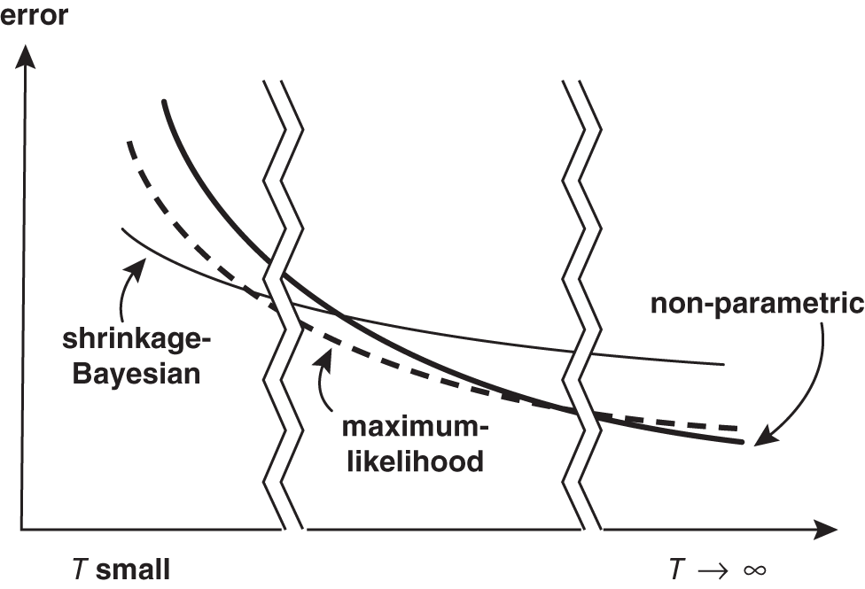
FIGURE 1.6 Estimation Error vs. Sample Size T (Reprinted with Permission from A. Meucci – ARPM Lab – www.arpm.co)
History repeating in the context of return distributions amounts to asking the question of whether the return distribution changes over time. Admittedly, we know that many assets both trend over short horizons and revert to the mean over intermediate term horizons; so we know over these horizons that history indeed does not simply repeat itself. But in the preface we made three assumptions, the first of which was that we were only interested in managing portfolios over long horizons. Therefore, the question of history repeating for our purposes is only relevant over multi-decade periods, which will generally hold for investable assets.
A distribution that is the same in one period of time as another period of time is formally called stationary. To test for stationarity we will provide a tool for comparing two return distributions to see whether they are similar enough to conclude that they are statistically the same. We will then use this tool to compare the return distribution from one multi-decade period to the next multi-decade period, to see if history indeed repeats itself. And in that process we will also provide the means to account for secular shifts over long-term horizons from effects like interest rate regime shifts.
At this point we still haven't addressed the question of sudden and irreversible changes to a return source that would make history irrelevant. Unfortunately we will not explicitly address this topic here, as it is beyond the scope of this book. Implicitly, though, by following the framework outlined in Chapter 3—which focuses on asset classes that have well-defined and logical risk premia—the intention is that we are only investing in assets whose return stream is expected to continue. For example, we assume that the compensation human beings demand for investing in companies (AKA the equity risk premium) is an invariant. In this book we always assume that the risk premia we choose to invest in will continue indefinitely.
The main takeaway here is that we will always attack the estimation problem head on and not try to obscure it or avoid it at any stage of our process. By investing in return sources that are stationary, and deploying large sample sizes for healthy measurement, we will be able to confidently utilize forecasts predominantly based on history.
We have just laid out a system for creating a joint return distribution estimate that is sensible (low estimation error) and we are now ready to push this forecast into our optimizer. But how sensitive to estimation error is the EU maximization process? Does the sensitivity preclude us from using models based on estimates that inevitably have errors altogether? And which estimates are the most critical for optimal performance of our portfolio? Are there specific moments we should focus on minimizing estimation error for?
The answer to all these questions is that it depends on the asset classes you are optimizing (Kinlaw, Kritzman, & Turkington, 2017). In general, there are two key takeaways on the topic of optimizer sensitivity to inputs. The first is that portfolios are more sensitive to means than variances (and higher moments) because utility depends linearly on returns but quadratically on variance terms (and cubically on skew, quadratically on kurtosis, etc.), as outlined by Eq. (1.4). Therefore, we need to ensure that our distribution estimate is completely buttoned up at the mean estimation level, by way of a large sample size, and then slowly relax the error bar requirements of our sampled distribution as we consider higher moments. While we are not directly estimating the mean or any higher moments in our process of estimating the entire return distribution, we are certainly implicitly doing so. Hence, in the process of estimating the entire return distribution, we will need to assess the accuracy of each moment estimate embedded in our full distribution estimate, and ensure our error bars are sufficient on a moment-by-moment basis. This issue will be fully covered in Chapter 4, alongside the rest of our discussion on sample size.
The second key takeaway on sensitivity to estimation error is that highly correlated assets generate much more input sensitivity in optimizers than less correlated assets. The return sensitivity seen in Figure 1.5 was largely attributable to the fact that large cap and small cap equities are highly correlated. Chapter 3 will address this sensitivity issue, where comovement effects are minimized by shrinking the universe of investments to the minimal set of orthogonal assets that still respects our client's utility function and their desired risk factor exposures. Note the careful use of “comovement” in the last sentence rather than covariance or correlation. The joint return distribution that is input into our optimizer considers not only linear comovements (covariance) but higher order comovements (coskewness, cokurtosis, etc.) as well. The method we review in Chapter 3 helps reduce sensitivity due to comovement, although it is greatly driven by linear comovement since it's a second order effect (as opposed to third or higher). Since the method includes higher order comovements as well, we must carefully shift to the more generalized terminology of comovement in that context.
Before we wrap up our discussion on the sensitivity to estimation error, let me make two quick points. First, there are a lot of solutions out there that address the error sensitivity problem by completely avoiding it. For example, the 60/40 prescription always allocates 60% to US equities and 40% to US bonds; while the 1/N portfolio equally invests in N assets. We will not consider these “heuristic” models for our clients, as they have zero connection with client utility or asset behavior. Second, there are a number of solutions that try to smooth the sensitivity to estimation error algorithmically, such as portfolio resampling, the Black–Litterman model,24 or robust optimization; but these models come at the cost of creating suboptimal portfolios,25 as they generally ignore higher moments and introduce mathematical complexities not suitable for an advisory practice. In this book we will solely look to address optimizer sensitivity to estimation error by tackling it head on with statistically sound sampling from history and avoidance of non-orthogonal assets.
It should be clear at this point that asset allocation should be defined as the process of maximizing a client's expected utility while minimizing the effects of estimation error. One should clearly not maximize utility with poor inputs, as the outputs to the process will not be relevant to future realizations of capital markets. At the other extreme, one should not accept a model that minimizes estimation error at the expense of ignoring client utility details or real-world asset behavior.
Hopefully, I have also substantiated the more explicit approach of maximizing a utility function with not one but three dimensions of client risk preferences while minimizing estimation error and its consequences by only investing in distinct assets and using statistically sound historical estimates as a forecast starting point.
This approach has a couple of key ramifications I want to reiterate briefly. First, we are completely committed to specifying each client's utility function, fully avoiding any approximation error at the problem specification stage. Specifying a utility function is not a common practice today, but with the right tools and a little training, it will provide an accurate and actionable assessment of risk preferences while providing advisors with a powerful framework with which to engage clients.
Second, the maximization of the full utility function requires returns-based optimization, where a forecast of all possible joint returns across assets is needed. This requirement moves us away from forecasting asset return moments, such as mean and variance, and into the business of forecasting the entire joint return distribution, which is just a long series of possible monthly returns for each asset. And it forces us to leverage historical data as much as possible, given the tremendously specific return outcomes required.
Third, estimation error and its consequences are addressed non-parametrically. This approach avoids any approximation error during forecasting and tremendously simplifies the estimation process for advisors. But it requires careful retort by users as to the statistical quality of the estimates (sample size) and the reasonableness of the assumption that history will repeat itself (stationarity). Additionally, advisors will dogmatically have to avoid any assets that do not qualify as orthogonal—a challenging responsibility in the world of asset proliferation and the desire to present a client with perceived value via complexity.
The remainder of this book will help advisors set up the process laid out in this section in a systematic and intuitive way. The process is certainly more intricate than other sub-optimal approaches, but my hope is that this optimal framework will ultimately be very accurate and intuitive to both advisors and their clients.
Let's now jump into step 1 of the four-step framework just laid out: setting the client risk profile.