
Equation 2.1 Formal Definition of SLR

In this chapter we take the first of four steps on our journey to finding a client's optimal asset allocation: setting the client's risk profile. The chapter begins with the careful measurement of client preferences regarding risk aversion, loss aversion, and reflection. Standard of living risk is then analyzed via a simple balance sheet model to help decide whether risk aversion and our two behavioral biases, loss aversion and reflection, should be moderated in order to meet the long-term goals of the portfolio. These two steps in conjunction will help fully specify our clients' utility function in a systematic and precise way.
Key Takeaways:
The simplest and most popular approach to establishing a client-specific risk profile is to measure volatility aversion by posing a series of qualitative questions on topics such as self-assessment of risk tolerance, experience with risk, passion for gambling, and time to retirement, and then using that score to choose a portfolio along the mean-variance efficient frontier at a risk level commensurate with the score. Unfortunately, there are three major issues with this process from the vantage point of this book. First, the typical risk tolerance questionnaire has a number of qualitative questions that are trying to pinpoint a very numerical quantity (utility second derivative), without a well-substantiated mapping from qualitative to quantitative.1 Second, the goals of the client are often analyzed qualitatively within the risk tolerance questions, without formal connection to well-defined retirement or multi-generational goals. And, third, this process has only been built to find a single parameter, uninteresting to us given our utility function that requires specification of three distinct risk preferences.
To address these issues, a concise two-step process is introduced. First, we present three lottery-style questionnaires, which precisely specify our clients' risk aversion, loss aversion, and reflection. We abandon the standard qualitative battery of questions, which convolutes different types of risk preferences and lacks a solid theoretical basis for mapping to utility parameters, in favor of our more numerate and surgical approach. Second, we deploy a simple balance sheet model to measure standard of living risk, which informs whether risk preferences need to be moderated in order to meet the client's goals. This model precisely accounts for standard lifecycle concepts, such as time horizon and savings rate, in a hyper-personalized manner while allowing us to avoid more complicated multi-period solutions.
We begin specification of our three-dimensional risk profile utility function (Eq. (1.8)) by measuring risk aversion γ, the neoclassical utility parameter that sets the second derivative of our utility function (AKA preference to volatility) if there is no loss aversion or reflection. To set this parameter systematically, we deploy a lottery-style questionnaire (Holt & Laury, 2002). Each question presents a simple binary gambling choice where you must choose between two options. Figure 2.1 shows a simple five-question version of this type of questionnaire that is explicitly designed to measure risk aversion. Each question poses a gamble to the client that, when aggregated together, can precisely determine the curvature of a power utility function. Preferences for the sure bet, which has a lower expected payout, map to a higher curvature utility function (more negative second derivative) and hence higher risk aversion while preferences to bigger payouts that are less certain map to a utility function with less curvature (less negative second derivative, noting that a straight line would have zero second derivative) and hence lower risk aversion. Note that these questions are explicitly written as a single gamble, not an opportunity to make the gamble repeatedly hundreds or thousands of times. This one-time phrasing aligns with the natural disposition for investors to be myopic (allowing short-term performance to influence their ability to stick with a long-term investment plan), as well our single-period representation of the portfolio decision problem as outlined in the preface.2

FIGURE 2.1 Risk Aversion Questionnaire
But how do the questions in Figure 2.1 help assign a precise risk aversion to a client? Seeing where a client decides to begin choosing Choice B allows us to set the risk aversion. If a client chooses Choice B for every question, they are clearly displaying little risk aversion. Clients who choose Choice A until question 4 or 5 are clearly more risk averse. Risk aversion is parameterized here between 1.5 and 12, as laid out in Figure 2.2.3 We show the percentage of the population that advisors can expect in each bucket based on these questions. In addition, Figure 2.2 shows the percentage of the population we would expect in each bucket if we multiplied the gamble sizes in our lottery questionnaire by 20 and actually paid out winnings. As you might expect, risk aversion shifts significantly higher when the gambles are real and 20 times greater in magnitude (these are known as “incentive effects”) (Holt & Laury, 2002). So, yes, we are now in a pickle. I have provided a small gamble lottery questionnaire that is completely hypothetical, which really doesn't elicit accurate subjective risk aversion results. And it turns out that it is not the 1x to 20x change or the hypothetical to real change that is responsible for this shift in risk aversion: it is the combination! I have never come across a wealth manager who elicits risk preferences with real gambling situations; but empirical testing has definitively shown us that this is the only way to measure true preferences.

FIGURE 2.2 Risk Aversion Mapping
What about the other possible permutations of answers besides the five shown in Figure 2.2? It has been shown that over 90% of respondents will be “consistent” and answer these questions monotonically, meaning once they flip their answer it will stay flipped. For those clients who do not answer in that way, it is useful for the advisor to insert herself and review the questionnaire with the client as an educational exercise. From a programmatic standpoint, my software utilizes the lowest question number where B is chosen to set ![]() (if B is never chosen, then risk aversion is set to 12) regardless of answers to higher question numbers. This approach sidesteps the monotonicity question, but still allows a client to answer non-monotonically. One could also tackle this issue programmatically by locking the answer choices to always be monotonic. For example, if someone chooses B for question 3, then questions 4 and 5 are automatically set to B; but then you would lose the additional color of a client misunderstanding the question as discussed above.
(if B is never chosen, then risk aversion is set to 12) regardless of answers to higher question numbers. This approach sidesteps the monotonicity question, but still allows a client to answer non-monotonically. One could also tackle this issue programmatically by locking the answer choices to always be monotonic. For example, if someone chooses B for question 3, then questions 4 and 5 are automatically set to B; but then you would lose the additional color of a client misunderstanding the question as discussed above.
In this section I have completely moved away from the style of risk questionnaire that has become popular over the past decade. Those questionnaires measure risk preferences in a number of different ways (self-assessment of risk tolerance, experience with risk, etc.) and in a more qualitative format than the gambling questions I have deployed here. Such a question might have a client rate their comfort level with risk among four choices (low, medium, high, very high). While there is indeed interesting research that explores the value of more qualitative and multi-dimensional questionnaires (Grable & Lytton, 1999) and of tying them explicitly to individual preferences or biases (Guillemette, Yao, & James, 2015), I have opted to pursue the more quantitative questionnaire path. My motivation to take this route is twofold.
First, I will always prefer a test that precisely maps to the thing we are trying to measure. In the academic world of questionnaire design, a test's ability to measure the intended feature is known as “validity” (Grable, 2017). Validity is generally tough to measure since we are typically trying to assess a quantity with no right answer we can compare to. Say you were creating an incredibly cheap clock and you wanted to make sure it was accurate. In that case, you have a great benchmark to test for validity: the National Institute of Standards and Technology (NIST) atomic clock.4 But in the case of risk preference assessments we have no such benchmark. What we do have is a precise definition of these parameters from our utility function, from which we can reverse engineer a series of questions that can help precisely measure the parameter. By performing this reverse engineering of the questions from the utility function, the hope is that we have near 100% validity (at least theoretically if a robot were answering it5).
You may be concerned at this point that we have traded improved validity for more challenging mathematical questions. It has been my experience that for most clients these more mathematical questions are quite straightforward, and they precisely elicit the emotional, gut reactions we are looking to ascertain in the process. Actually, it is usually the advisors who struggle more with these questions as they may view the questionnaires as more of a test, which inevitably leads them to wonder whether they should make decisions based less on the emotional nature of risk aversion and more on expected value. While this behavior is less frequent in clients, it will certainly come up for more financially literate clients, and advisors should be prepared to recognize this rabbit hole situation and steer clients toward a more emotional response to the questions. Ultimately, I am very hopeful that these more quantitative diagnostic questions will represent a welcome component to the advisor's engagement with the client while preserving the precision of what we are trying to achieve.
Second, the simplest path for me to take in diagnosing both loss aversion and reflection was through lottery-style questions similar to those presented here for risk aversion. In an effort to stay consistent with the style of questionnaire deployed for setting all three utility features, I then had to stick with lottery-style for the risk aversion feature. At the end of the day, as long as a risk parameter questionnaire is rigorously tested for validity, and the limits of the test are well understood by the advisor, I believe the exact style of the questionnaire is flexible and can be guided by the real-world usage.
Before we move on from risk aversion, let me briefly mention that it has been shown that risk aversion changes in time for investors: they are more risk-averse after losses (“break-even effect”) and less risk-averse after wins (“house money effect”) (Thaler & Johnson, 1990).6 It is thus very useful for an advisor to periodically measure their client's risk aversion to account for this effect, and to educate their client on the topic (the same periodic check-in should be done for loss aversion and reflection as well). But which risk aversion do you deploy if you're regularly measuring it and it is changing in time? You want to use the level that is established during average market environments, avoiding the break-even and house money effects altogether. Both of these effects are due to the component of prospect theory that we have ignored (see “decision weights” in footnote 17 of Chapter 1), and as such, we do not want to unwittingly introduce it into our process.
In Chapter 1 we showed that the first behavioral deviation from neoclassical utility we want to consider is loss aversion, coded into client risk preferences by assigning a value for ![]() in our utility function (Eq. (1.8)) that deviates from 1. This parameter ascertains an irrational asymmetric discomfort of downside versus upside moves, greatly influencing portfolio preferences regarding drawdowns. To precisely assess one's degree of loss aversion, we will continue to deploy lottery-style gambling questions (Gachter, Johnson, & Herrmann, 2007). Such a question for loss aversion might ask: Would you accept or reject a lottery where a coin is flipped and the payout is −$1 when tails comes up and +$2 when heads comes up? If you say no to this, then we can conclude you have some degree of loss aversion. Why is that so? First, the question refers to both losses and gains, stepping us away from the arena of risk aversion where all possible outcomes were gains, and into the world of loss aversion which measures our preferences for gains versus losses. Second, we are avoiding the background curvature given by our utility function's risk aversion by only considering bets that are small enough to ensure that the utility function is effectively linear between the two outcomes7—which turns the problem into a pure expected return problem (which any rational investor would accept in this specific instance). Hence, if you reject this particular lottery, you are showcasing a bias to loss aversion. But how do we take a short list of questions like the one above and turn them into a score?
in our utility function (Eq. (1.8)) that deviates from 1. This parameter ascertains an irrational asymmetric discomfort of downside versus upside moves, greatly influencing portfolio preferences regarding drawdowns. To precisely assess one's degree of loss aversion, we will continue to deploy lottery-style gambling questions (Gachter, Johnson, & Herrmann, 2007). Such a question for loss aversion might ask: Would you accept or reject a lottery where a coin is flipped and the payout is −$1 when tails comes up and +$2 when heads comes up? If you say no to this, then we can conclude you have some degree of loss aversion. Why is that so? First, the question refers to both losses and gains, stepping us away from the arena of risk aversion where all possible outcomes were gains, and into the world of loss aversion which measures our preferences for gains versus losses. Second, we are avoiding the background curvature given by our utility function's risk aversion by only considering bets that are small enough to ensure that the utility function is effectively linear between the two outcomes7—which turns the problem into a pure expected return problem (which any rational investor would accept in this specific instance). Hence, if you reject this particular lottery, you are showcasing a bias to loss aversion. But how do we take a short list of questions like the one above and turn them into a score?
For precise score measurement we will again deploy a sequence of lottery questions, which directly implies a loss aversion score when analyzed as a whole. Figure 2.3 outlines four questions that follow a simple sequence of increasingly risky bets. The basic idea here is similar to what we just deployed to measure risk aversion, except now losses are involved: each lottery has larger losses as we go down the list, and the point at which someone begins to reject the lottery pinpoints their loss aversion precisely. The earlier in this sequence of gambles that a client begins to reject the lottery, the more loss averse they are, given that all bets are completely rational from an expected utility standpoint: they are all just expected value decisions, as reviewed in the previous paragraph.
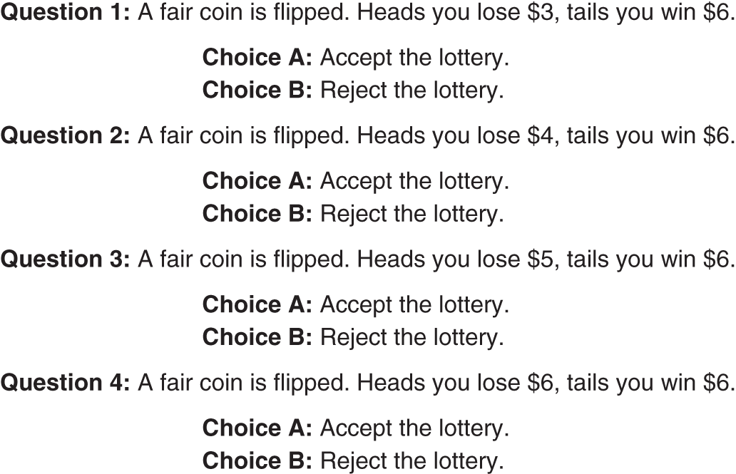
FIGURE 2.3 Loss Aversion Questionnaire
For the remainder of this book, ![]() is parameterized between 1 (no loss aversion) and 3 (maximal loss aversion), aligning with modern research on the subject that shows clients often have loss aversion between these levels (Gachter, Johnson, & Herrmann, 2007). The exact mapping from lottery rejection point to
is parameterized between 1 (no loss aversion) and 3 (maximal loss aversion), aligning with modern research on the subject that shows clients often have loss aversion between these levels (Gachter, Johnson, & Herrmann, 2007). The exact mapping from lottery rejection point to ![]() is laid out in Figure 2.4. As you can see,
is laid out in Figure 2.4. As you can see, ![]() is just the ratio of win versus loss magnitudes where the questionnaire is last accepted—a 100% valid mapping of questionnaire to preference that is much more transparent than the mapping for risk aversion (which requires additional utility mathematics). Figure 2.4 also shows expectations for how clients should roughly be distributed across the bins.8
is just the ratio of win versus loss magnitudes where the questionnaire is last accepted—a 100% valid mapping of questionnaire to preference that is much more transparent than the mapping for risk aversion (which requires additional utility mathematics). Figure 2.4 also shows expectations for how clients should roughly be distributed across the bins.8
Finally, similar to the risk aversion questionnaire, around 90% of respondents will answer monotonically (i.e. once the client flips to Choice B they will continue to do so for the rest of the questions). Similar to what we did for risk aversion, my software utilizes the lowest question number that is rejected to set ![]() , regardless of answers to higher question numbers, hence sidestepping the monotonicity question.
, regardless of answers to higher question numbers, hence sidestepping the monotonicity question.
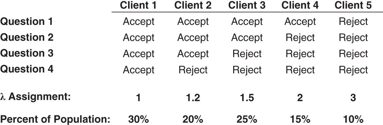
FIGURE 2.4 Loss Aversion Mapping
The second deviation from a purely rational utility function we need to assess is reflection. As a reminder, this feature is captured by our three-dimensional risk profile utility function (Eq. (1.8)) via the specification of reflection ![]() that departs from 0, informing us that a client has an irrational preference to become risk-seeking when contemplating losing positions. But in contrast to risk aversion and loss aversion, which are captured by variable parameters in our utility function, reflection is a binary variable that can only take on the value 0 or 1. As mentioned in Chapter 1, we could have parameterized reflection further by setting the curvature of the S-shaped function differently in the domains of losses and gains. But to help facilitate an intuitive interpretation of our utility function that translates well to clients, we have opted to keep things simple and just flag reflection as existing or not.
that departs from 0, informing us that a client has an irrational preference to become risk-seeking when contemplating losing positions. But in contrast to risk aversion and loss aversion, which are captured by variable parameters in our utility function, reflection is a binary variable that can only take on the value 0 or 1. As mentioned in Chapter 1, we could have parameterized reflection further by setting the curvature of the S-shaped function differently in the domains of losses and gains. But to help facilitate an intuitive interpretation of our utility function that translates well to clients, we have opted to keep things simple and just flag reflection as existing or not.
So how do we diagnose reflection in our clients? For this we utilize the question set shown in Figure 2.5, which asks the exact same question twice, once in the gain domain and once in the loss domain.9 There are four possible combinations of answers a client can choose during this questionnaire: Choices A and 1, Choices A and 2, Choices B and 1, and Choices B and 2. The only combination set of the four that indicates reflection ![]() is the second (Choices A and 2), as we see the client opting for the risk-averse option in the gain domain and the risk-seeking option in the loss domain. None of the other three answer combinations would be consistent with reflection. Hence, we say a client showcases reflection if and only if Choices A and 2 are chosen by the client. In terms of expectations of our clients for reflection, we expect about half of them to be flagged for the reflection bias (Baucells & Villasis, 2010).
is the second (Choices A and 2), as we see the client opting for the risk-averse option in the gain domain and the risk-seeking option in the loss domain. None of the other three answer combinations would be consistent with reflection. Hence, we say a client showcases reflection if and only if Choices A and 2 are chosen by the client. In terms of expectations of our clients for reflection, we expect about half of them to be flagged for the reflection bias (Baucells & Villasis, 2010).

FIGURE 2.5 Reflection Questionnaire
Many readers might wonder at this point whether the question set in Figure 2.5, which only contains two questions, is sufficient to diagnose a client's reflection. This is an excellent question; it is essentially asking what the measurement error is for each of the four answer combinations (it is the number of distinct answers that matters more than the number of questions, in terms of diagnostic accuracy). And the same exact question must be asked regarding our risk and loss aversion questionnaires (six and five distinct answers, respectively). We are now entering the domain of questionnaire “reliability” (Grable, 2017).
Besides validity, reliability is the other key requirement of a healthy questionnaire, as it measures how repeatable the results are for a given individual. In other words, it measures the inverse of the questionnaire's measurement error. Said another way, validity measures systematic deviations for every participant in the test, whereas reliability measures the variance around individual respondent answers. An easy way to remember the difference between these two concepts is by thinking of a linear regression from Stats 101, where we always assume the data points we are regressing are perfectly measured (there are no error bars on the data points themselves, AKA reliability is 1), and we analyze whether a linear model is a good representation of our data (i.e. is valid) via R2 (which runs from 0 to 1).
We can also gain a little more clarity on reliability if we understand how it is measured. There are many ways to do this, but one popular method is to ask the same question to the same person at different points in time and look at the correlation of the answers (i.e. a “test-retest” reliability procedure). A correlation of 1 indicates perfect reliability. Although reliability of questionnaires is of paramount importance, the topic is generally considered to be outside the purview of this book, as it is an entire field in and of itself. For now I simply assume perfect reliability for our questionnaires since we have four or more distinct answers for each questionnaire (and not just one or two, which would worry me more).
We have presented three lottery-style questionnaires designed to measure each utility function parameter accurately. As briefly reviewed for risk aversion, empirical work has shown that the sizing of the questions has a big impact on the responses, where smaller gambles will generally elicit lower risk aversion. Additionally, we saw that loss aversion questions need to be posed with very small gambles. So how do we size all these questions appropriately? There are three key issues at work when sizing the gambles.
The first is that loss aversion is a concept that must be carefully measured without any influence from the curvature of the utility function. Hence, loss aversion gambles should be sized significantly smaller than the risk aversion or reflection questions, which are both squarely related to curvature of utility. The second key constraint is that the loss aversion question must have gamble sizes that are meaningful enough for a client to take the question seriously. If you ask someone worth $50 million about winning or losing a single dollar, the question may be treated the same as if they were gambling with dirt, with zero connection to their true emotional preference. Finally, the risk aversion and reflection questions should be sizable enough to actually measure utility curvature (the opposite situation we are in for loss aversion), and in agreement with the earlier results showing that smaller gambles in risk aversion questions will not elicit true preferences.
To facilitate all three effects one could base the gamble size in the risk aversion and reflection questions on a client's annual income, and then appropriately scale down the loss aversion gamble sizes from there, but not too much. In my software I test clients with risk aversion and reflection gambles that are 1/200th of annual income while I deploy loss aversion gambles that are 10 times smaller than that. For example, a client with annual income of $200,000 would answer risk aversion and reflection questions in the $1,000 ballpark while answering questions on loss aversion near $100, an intuitively reasonable solution to our three priorities regarding gamble sizes.
Now that we have measured the three preferences embedded in our client's utility function, are we finished specifying our client's risk profile? Not exactly. It turns out that if you account for the goals of the portfolio, you are naturally confronted with the fact that you may need to moderate (i.e. override) the three parameters of the utility function we have carefully measured.
Up to this point in the book we have deployed assumptions that allow us to focus on the single period portfolio problem of maximizing the following month's expected utility. In addition, we have completely ignored any long-term goals of the portfolio that would require a multi-period framework. But we know our clients indeed have goals for their portfolios. For most of us the goal is to have enough wealth to survive during retirement. For wealthier individuals the goal might be a sizable inheritance for their children. So how do we incorporate goals into our process in a systematic way while still being able to focus on the simplified single-period expected utility problem?
The key here is to realize the following: when we introduce goals, risk taking changes from being a personal preference to a luxury that we may or may not be able to afford. In other words, low risk aversion may need to be moderated if our client's balance sheet isn't able to take on a lot of risk when considering their goals.10 An extreme example would be a client whose goal is to withdraw tomorrow $100,000 from an account that is currently worth that amount today. Clearly, this client cannot put any risk in the portfolio, or they jeopardize meeting their goal if the portfolio has a down day. Hence, if the portfolio goal is risky but the client has low risk aversion, the preference for risk aversion must be moderated upwards. In effect, if we have a goal in mind that we want executed with certainty, we must start off with a risk-free portfolio, and only if our goals are easily achievable can we then take on more risk. Said another way, risk is a luxury.
What about the financial plan that “gets” a client to lofty financial goals with markedly less than 100% certainty? If your goal is flexible, then yes, you can set out a goal that may not be achieved which can then be updated after failure, but in this book we will be focused on the hyper-fiduciary mission of building portfolios with inflexible goals. We will return to this topic when we discuss Monte Carlo simulations of future expected wealth and how these tools can help us add some flexibility to the plan as long as risk preferences are respected and there is some flexibility in goals. With that said, this book generally recommends the more risk-controlled, goal-focused process that assumes that financial goals are first-and-foremost inflexible, and that risk should only be deployed in portfolios when one can sufficiently meet their goals with certainty (i.e. without risky investments).
We will refer to the riskiness of meeting one's portfolio goals as standard of living risk (SLR) (CFA Institute, 2018). One may loosely think of SLR as an inverse measure of the probability of meeting your goals, where lower SLR represents higher probability of meeting your goals and higher SLR represents lower probability of meeting your goals. When SLR is high, as it was in our $100,000 example above, risk aversion will need to be moderated upwards. When SLR is low, we will let the client's natural risk aversion dictate the riskiness of the portfolio.
Many of you will have heard of the term risk capacity, a measure of how much risk your goals can handle. If you have, you may also have heard that you don't want your client's risk tolerance (1/risk aversion) to be higher than their risk capacity. This is the exact same system we are discussing here, except this nomenclature inverts the scales of the risk parameters we deploy (SLR is proportional to 1/risk capacity). You may have also seen the phrasing “subjective versus objective risk aversion,” where subjective risk aversion is the client preference and objective risk aversion is proportional to 1/risk capacity—where one always wants to ensure the client's portfolio is deployed using the higher of the subjective and objective risk aversion scores.11 This is the same framework we have put forth here on moderating risk, just with modified lingo that we will deploy within this book when useful.
What about our two behavioral parameters? The same simple concept applies to behavioral biases as well but from a slightly different perspective. The two behavioral preferences we encapsulate in our utility function are both suboptimal when it comes to long-term wealth optimization, and hence are a form of luxury that isn't available to someone who is not likely to meet their goals. Hence, we will moderate both loss aversion and reflection when SLR is high—not because we are taking on too much risk, but rather because we can't afford any sub-optimality. The situation for behavioral biases is even more subtle than that and is worth a short digression.
Moderation of behavioral biases can be conveniently summarized by the framework shown in Figure 2.6.12
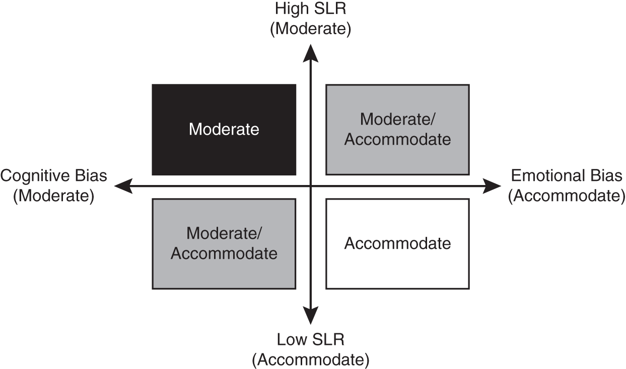
FIGURE 2.6 Moderation vs. Accommodation of Behavioral Biases
Beyond enforcing greater moderation of behavioral biases as SLR increases, the framework also recommends advisors should be less compromising with cognitive biases than they are with emotional biases. The rough idea here is that emotional biases are driven by subconscious responses which are difficult to rectify, which may warrant adaptation to stick with a plan, while cognitive biases are driven by faulty reasoning or a lack of information, which should only be moderated. Why not just tell your client how to behave rationally and that is all?
The premise here is simple: a sub-optimal plan your client can actually follow is better than an optimal plan your client can't follow.13 In other words, a slightly lower utility portfolio adhered to is better than a portfolio with higher utility that is not adhered to, if your goals can handle such accommodation. A perfect example is the Great Recession. Many clients had portfolios optimized for their risk tolerance, but the portfolio wasn't built with their behavioral biases in mind, and many of these clients got out of the markets at the bottom and didn't reenter until many years later. These clients were much better off in a portfolio that might be sub-optimal for a fully rational investor but one that if adhered to would be much more beneficial than being in cash for extended periods. Fortunately, both components of PT that we account for via our three-dimensional risk profile utility are emotional biases and the two-dimensional framework collapses to a simpler one-dimensional tool that is just a function of SLR; hence, we have the same situation as we do for moderating risk aversion: we will moderate irrational behavioral biases when SLR is high.
What about the litany of other emotional biases that researchers have discovered over the past 50 years (Pompian, 2006)? Why aren't they accounted for in our utility function? It turns out that there are a number of emotional biases that are not relevant for our usage here, or the effect is subsumed by loss aversion and reflection. For example, self-control bias is an important emotional bias tied to one's inability to consume less now for rationally smoothed long-term consumption. While we indeed spend time discussing how the single period problem should be translated into a retirement solution, we assume that self-control bias can be overcome with modern fintech such as automated savings programs.
As another example, consider the endowment bias (a direct consequence of PT), where investors get emotionally tied to individual holdings and have difficulty parting ways with them. In this book we assume clients are not wedded to any positions, by assuming clients have a more distant relationship with their investment portfolios, a trend we only see continuing. Additionally, at the portfolio level the endowment effect is captured by loss aversion, which implies favoring of the status quo (i.e. you won't take a 50/50 bet with equal absolute payoffs).14 There are many more biases we could cover in this way, but you will just have to trust me that if you first weed out the emotional biases from the cognitive ones, and then remove those biases that don't affect our use case, any biases remaining will be subsumed by reflection and loss aversion.
With the asymmetric view that we will lower risk for a goal but never raise it, and the fact that our two behavioral biases should be moderated as well when goals are lofty due to their sub-optimality, we have hopefully accomplished our intention of the section—to advocate the moderation of all three utility parameters when the goals of the portfolio are increasingly at risk of not being met. In the next section we introduce discretionary wealth as a simple yet powerful way to measure SLR. This tool enables us to moderate our three utility parameters in a systematic yet personalized manner, and ultimately to provide a goals-conscious asset allocation solution.
To measure SLR we move away from the lottery-based questionnaires and shift to a balance sheet model that can easily capture the client's goals and the risk associated with achieving them. On the left side of the balance sheet is a client's implied assets, which includes both assets currently held and the present value (PV) of all future assets. For our current purposes, we will have only three items on the asset side of the balance sheet: the client's investment portfolio, the value of their home, and the PV of all future savings through employment (i.e. PV of future employment capital minus spending). On the right-hand side of the balance sheet is today's value of all current and future liabilities. In our simple model this will include the client's total current debt (typically school loans and/or a mortgage) and the PV of all expected spending needs during retirement. Figure 2.7 shows the balance sheet model for a client with a $1 million home, a $500k investment portfolio, and a $500k PV of all future savings before retirement. This compares to liabilities of $0 of current debt and a PV of required capital for retirement of $1 million.
So how do we tease SLR out of this model? The key is the client's discretionary wealth (Wilcox, Horvitz, & diBartolomeo, 2006),15 which is simply total implied assets minus total implied liabilities—that is, total net implied assets. What is this number exactly and how does it help us? Simply said, discretionary wealth is the wealth you don't need. More precisely, it tells you how much money you have left after all your current and future obligations are met by only investing at the risk-free rate. If discretionary wealth is high, then your assets are ample to meet liabilities and you indeed have the luxury of deploying risk in your portfolio. If it is low, then you have very little padding in your financial situation and you don't have the luxury of taking on much risk. Hence, discretionary wealth is the perfect metric to help us assess whether someone's retirement goals are at risk. In the example given in Figure 2.7 we have discretionary wealth of $1 million, a favorable position for our client, and one that should afford them the luxury to take on risk in their investment portfolio.

FIGURE 2.7 Balance Sheet Model
Let's now move to formally mapping discretionary wealth to SLR. First let's distinguish two key regimes of discretionary wealth: greater than 0 and less than 0. When discretionary wealth is less than zero, we have a problem. The balance sheet model is telling us that even if we invest in the risk-free asset, our client will not achieve their goals. In this case, the client's balance sheet must be modified via some tough conversations. To move discretionary wealth into positive territory a client can take certain actions such as working longer, increasing their savings, reducing their income level in retirement, and minimizing liabilities.
Once our client is in positive discretionary wealth territory, we note that the ratio of discretionary wealth to total implied assets will always lie between 0% and 100%, which is a great indicator of a client's current financial health. If a client has a 0% ratio of discretionary wealth to total assets, then they are just squeaking by to meet their financial goals and have zero ability to take on risk. On the other extreme of the spectrum, a 100% ratio means the client has zero liabilities relative to assets and can take on as much risk as they would be interested in accepting. To map this ratio to SLR is now simple:
Equation 2.1 Formal Definition of SLR
Once discretionary wealth is greater than 0, SLR will always lie between 0 and 100%, a very simple and intuitive range for measuring standard of living risk. In our case study in Figure 2.7 our client's $1 million of discretionary wealth maps to an SLR of 50%, perhaps a slightly less favorable number than you might expect given the impressive absolute level of the discretionary wealth. This outcome highlights that it is not the absolute level of discretionary wealth that matters, but rather the ratio of discretionary wealth to total implied assets, since the health of a certain level of discretionary wealth is irrelevant without a full comprehension of how the discretionary wealth compares to the ultimate liabilities. Even a large discretionary wealth isn't that attractive if the liabilities are incredibly large since one's level of padding is all relative!
The last step of moderating our three utility preferences is to use SLR, as defined by Eq. (2.1), to adjust our risk and behavioral parameters measured by our lottery-style questionnaires. Our SLR will have us maximally moderating at 100% and not moderating at all at 0%, but the precise approach for systematically moderating preferences via SLR will be different for each parameter. Let me note upfront that the precise details for the moderation system presented below is an intuitively reasonable framework, but I am sure it can be improved upon, and I encourage others to put forth more advanced logic around the precise moderation rules.
For risk aversion, we map the SLR scale of 0–100% to a score from 1.5 to 12 and then set our risk aversion parameter to be the greater of the measured risk aversion and this SLR-based “objective” risk aversion. Hence, if a client has plenty of risk tolerance in the form of a risk aversion of 3, but his SLR is 50% (mapping to an objective risk aversion of 6.75), then the γ of our utility function is set to 6.75 (the higher of the two). This moderation rule, along with the rules for loss aversion and reflection that we are about to review, are summarized in Figure 2.8.
To reiterate, when SLR hits 100%, we are moderating to a very low-risk portfolio (![]() is not completely risk-free, but one could update this system to moderate to a completely risk-free portfolio). By moderating to a minimal-risk portfolio we are effectively guaranteeing that we will meet our liabilities. As described in the beginning of this section, our moderation process is very risk-focused, putting success of financial goals above all else (while respecting any immutable risk aversion).
is not completely risk-free, but one could update this system to moderate to a completely risk-free portfolio). By moderating to a minimal-risk portfolio we are effectively guaranteeing that we will meet our liabilities. As described in the beginning of this section, our moderation process is very risk-focused, putting success of financial goals above all else (while respecting any immutable risk aversion).
For loss aversion we will do something similar but now our directionality is flipped. We map SLR to a score from 3 to 1 as SLR moves from 0 to 100%, and we set ![]() deployed in our utility function as the lower of this SLR-mapped loss aversion number and the measured preference. For instance, if our client has a subjective
deployed in our utility function as the lower of this SLR-mapped loss aversion number and the measured preference. For instance, if our client has a subjective ![]() of 3 and an SLR of 50% (mapping to an “objective”
of 3 and an SLR of 50% (mapping to an “objective” ![]() of 2), we will moderate loss aversion down to the objective score of 2.
of 2), we will moderate loss aversion down to the objective score of 2.

FIGURE 2.8 Preference Moderation via SLR
Finally, we must moderate those clients that exhibit a reflection bias while having a high SLR. Since reflection for us is not continuous, we must choose an SLR level to discretely moderate our client from an S-shaped utility ![]() to a power or kinked functional form
to a power or kinked functional form ![]() . For the remainder of this book we will assume an SLR of 50% or greater to represent a reasonable level of discretionary assets where reflection should be discretely moderated. In this way we have planted our flag in the sand that SLR of 50% is a reasonable tipping point for us to take the viability of our goals very seriously and begin to completely abandon any suboptimal binary biases. This rule will become better motivated in Chapter 5 when we see how our portfolios evolve as a function of our three parameters, and how moderation of preferences by SLR will impact portfolios.
. For the remainder of this book we will assume an SLR of 50% or greater to represent a reasonable level of discretionary assets where reflection should be discretely moderated. In this way we have planted our flag in the sand that SLR of 50% is a reasonable tipping point for us to take the viability of our goals very seriously and begin to completely abandon any suboptimal binary biases. This rule will become better motivated in Chapter 5 when we see how our portfolios evolve as a function of our three parameters, and how moderation of preferences by SLR will impact portfolios.
An interesting question might come up for you at this stage: Should we ever accommodate very extreme cases of behavioral biases even when SLR is near 100%? In theory, one could indeed do this by engaging in the incredibly challenging conversation of lowering SLR down to the 0–25% range by dramatically changing the client's goals. However, given the magnitude of the ask to bring SLR down so significantly, it will in general be a lot more reasonable to moderate the biases while only having to bring SLR to 75% or so.
The purpose of the SLR definition presented here was to provide a succinct and completely systematic tool to moderate three distinct preferences in an effort to achieve given financial goals. This system rested on a strong premise, that financial goals should be paramount and 100% success rates were a driving factor behind the system. Let's now review other tools commonly used when moderating preferences for goals and see how they stack up.
Many advisors today deploy Monte Carlo simulations to investigate whether goals are likely to be reached. In that setting an advisor analyzes all possible cash flow outcomes over long horizons by running simulations of all possible expected capital market paths. By then looking at the portfolio's success rate, which is the percentage of simulated portfolio paths that achieve the desired cash flow goals, the advisor can then iteratively moderate the recommended asset allocation or goals (or even worse, preferences) until an acceptable solution is found, with typically acceptable success rates near 70% or so. The main challenge to deploying this process in our three-dimensional risk preference framework is that we are no longer just dialing up or down the risk of the portfolio and the related width of the Monte Carlo end-horizon outcome set. In our framework, we must moderate three distinct preferences, one of which (loss aversion), is generally moderated toward higher risk portfolios when SLR is high due to the suboptimal nature of highly loss-averse portfolios. An a priori system such as that laid out in Figure 2.8, rather than an iterative, ex-post system to set portfolios and goals such as Monte Carlo simulations, is much more necessary in a more nuanced utility function framework that incorporates both rational and irrational behaviors that moderate in different directions of riskiness. With that said, one can certainly manually modify the portfolio slowly using the three-dimensional map of optimal portfolios reviewed in Chapter 5, and rerun Monte Carlo simulations to finalize a portfolio plan; but the SLR-based moderation system should be a welcome systematic starting place for the process.
As mentioned earlier, one main lever advisors rely on when quoting success rates below 100% is the “flexibility” of the earnings and consumption assumptions baked into the simulation. These goals can indeed be adjusted as time goes on if the client is young enough and open to potential downgrades in future standard of living. I dogmatically avoid this downgrade risk and instead focus on leaving open the opportunity for a standard of living upgrade if the capital markets and savings paths realized are favorable. Of course, as long as the flexibility argument and the potential for failure are clearly presented to the client and well documented, this is certainly a reasonable conversation to have with your client, and one that will certainly require accurate Monte Carlo simulations for proper assessment.
Monte Carlo simulations are a fantastic tool to help understand the variability of future possible wealth outcomes, but I view these as ex post analytics that help verify our ex ante SLR process, or can be used to assess flexibility arguments. In other words, this book recommends starting with what is essentially a straight-line Monte Carlo result (a risk-free investment whose path is totally deterministic) and slowly opening our client portfolios to risk as SLR drops from 100%, with minimal iteration and with near 100% success rate. And when flexibility of goals is on the table, Monte Carlo simulations will bring a relevant layer of information to the advisor's process.
Hopefully, it is now clear that our definition of SLR and how we have translated that into our utility function naturally and explicitly incorporates most of the familiar balance sheet concepts, such as time horizon, goals, human versus financial capital, and so on. But how does this framework compare with the typical glidepath solution?
For those not familiar, a glidepath is a prescribed asset allocation that changes in time assuming you are retiring in X years. There are many different glidepath methods out there, but the best ones I've seen look to maximize income at retirement while minimizing income volatility near retirement (i.e. they maximize ending utility of income) (Moore, Sapra, & Pedersen, 2017). Many of these systems will also account for the volatility of human capital and correlations of human capital with financial assets.
So a typical glidepath solution is similar in the objective it is maximizing to what we are focused on here.16 However, glidepaths account for human capital as an investable asset while being completely void of any personalized financial goals, whereas, our discretionary wealth framework is squarely focused on achieving a client's personal financial goals without considering the stochastic nature of human capital.
When calculating the tradeoff between a system that includes human capital as an explicit asset but is ignorant of personal cash flow goals, and one that ignores the risk characteristics of human capital yet is cognizant of personal financial goals, I have obviously opted for the latter. This is for three reasons: (1) I believe meeting retirement goals is paramount to any other considerations (as is probably evident from the advocated moderation system focused on a 100% success rate); (2) I want to keep the solutions here simple, confining the discussion to the domain of the single period problem (the glidepath solution is inherently multi-period); and (3) most glidepaths assume bond-like human capital, which is effectively what we are assuming in our discretionary wealth framework. Ideally, we will someday bring the riskiness of human capital into this simplified balance sheet solution, but for now we will stick with our compact SLR approach, due to its simplicity and more stringent focus on achieving a desired standard of living in retirement or multi-generational wealth transfer.
In terms of the difference you can expect between a typical glidepath solution and ours, one must first ask how volatile the human capital is assumed to be in the glidepath approach.17 On the one hand, very volatile human capital (e.g. that of a commodity trader) would require investors to start with very little equity exposure early in their career, which rises in time. On the other hand, low volatility human capital (e.g. that of a tenured professor) would push an investor into higher equity allocations early on, which slowly decrease. As previously noted when justifying our choice of the simpler single-period lifecycle framework, the typical glidepath assumes low volatility human capital, and so we can expect a steadily declining equity allocation from these models into retirement.
Our balance sheet model, on the other hand, is dominated by whether someone is saving properly for retirement. Our most frugal clients will have the lowest SLR (highest equity allocations), as they save aggressively and keep retirement spending goals low. Our least frugal clients will have high SLR's and low equity allocations. For example, a young worker with a reasonable savings plan should be afforded a decent amount of risk early on, given their long stream of expected assets and a liability stream that is so far out that the PV is currently minimal. As liabilities approach closer to one's horizon, discretionary wealth will go down and SLR will rise, and a lower risk portfolio will become more appropriate. Hence, in the case of a “rational” worker with a thoughtful plan for preserving their standard of living in retirement, our client will have an equity allocation in time that looks similar to the typical glidepath. Our framework stands out, though, for people who don't fit nicely in this bucket, where a glidepath solution would certainly let them down due to their less responsible habits. It is the customizable nature of this model that presents the most value.
If you think about it further, our lifecycle model effectively maps the glidepath's human capital riskiness to the risk of being underfunded in retirement (since we have assumed that human capital is bond-like). Most people have steady incomes for employment but are challenged on the saving/spending side of the equation; hence, this swap of focus from human capital riskiness to SLR should be a welcome transition for any wealth management practice.