
Equation 5.1 2nd Order Approximation of Our Three-Dimensional Utility Function
CHAPTER 5
Portfolio Optimization
Step 4 of four in our asset allocation process brings us to our crowning moment: running an optimizer to produce portfolios that respect nuanced client preferences while simultaneously being robust to estimation error. The chapter begins with a review of our optimizer results as a function of our three-dimensional client risk profile space, showcasing an intuitive evolution of portfolios as our three preference parameters change. We then spend time contrasting our framework with other potential solutions to elucidate the value of our three-dimensional risk preference utility functions. The chapter ends with a review of the sensitivity of our recommended portfolios to estimation error, as we deploy the bootstrap method to create error bars on each asset's recommended allocation.
Key Takeaways:
- Our modern utility function results in an intuitive three-dimensional landscape of optimized portfolios that is rich in behavioral content.
- The three-dimensional utility function is a critical requirement for systematic incorporation of financial goals into a PT-conscious asset allocation framework, even when higher moments are not meaningful.
- The error bars on our optimizer's recommended portfolio allocations are large but manageable, highlighting the importance of always minimizing estimation error and its consequences.
- Our asset allocation error bars go down as we expand our outcome forecasting sample size, and as we limit redundancy of asset classes, validating our deployment of these techniques for this purpose.
INTRODUCTION
This book has promised a modern yet practical solution to the asset allocation problem within wealth management. On the modern side, we promised an advanced client profile, defined by a utility function with three risk preference parameters, and an intelligent balance sheet moderation system of these preferences. On this front, we also deployed a returns-based expected utility optimization routine that can account for higher order moments of the assets we invest in. On the practical side, we promised a solution with reasonable estimation error and lower estimation error sensitivity. To this end, we deployed non-parametric estimation from historical data with large sample sizes, alongside an asset selection process that minimizes estimation error sensitivity by avoiding redundant assets, so that our optimizer could be run without unnecessary sensitivity to inputs or manually imposed allocation constraints. It is now time to run our optimizer and see if the pieces we have put in place result in an investment solution that delivers on our promises.
The chapter begins with a review of the portfolios recommended by our modern utility function. We will see an intuitive evolution of risk-taking as we traverse the three-dimensional space defined by the three risk behaviors we are accounting for. We then compare our framework with other possible solutions to drive home the key benefits of our modernized three-dimensional risk profile system: a client profile rich in intuitive behavioral content, and the ability to incorporate financial goals systematically when human behavior is properly accounted for.
We then move on to the practical side of our framework, designed to address the challenges of optimizer sensitivity, which pushes many advisors away from using optimizers and into generic heuristic methods. We will deploy the bootstrap method once again, this time sampling with replacement from the full history of joint distributions when feeding outcomes into our optimizer. This creates error bars on our recommended asset allocation results that will help inform whether our framework is indeed helping reduce estimation error and the sensitivity to it. We will see our recommended techniques of deploying assets with low mimicking portfolio tracking error (MPTE) and large sample size successfully help us improve our asset allocation error bars.
OPTIMIZATION RESULTS
Figure 5.1 shows our returns-based optimization results for our chosen asset classes (for simplicity, without our equity and duration geographic risk premium (GRP)). We deploy our full 1972–2018 joint return distribution as our forecast, with no tax, fee, or other adjustments, and only show a subset of ![]() and
and ![]() values, again in an effort to keep the presentation simple.1 There are four key takeaways the reader should glean from the menu of portfolios in Figure 5.1, which should both validate the framework we have developed in this book and provide refined intuition for how the framework can be deployed across a wide client base.
values, again in an effort to keep the presentation simple.1 There are four key takeaways the reader should glean from the menu of portfolios in Figure 5.1, which should both validate the framework we have developed in this book and provide refined intuition for how the framework can be deployed across a wide client base.

FIGURE 5.1 Optimization Results for Selected  ,
,  , and
, and 
First, the resulting portfolios demonstrate an intuitive evolution of portfolios as we navigate through the three-dimensional space of client risk parameters. Higher risk aversion, higher loss aversion, and lower reflection all lead to portfolios with lower allocations to performance assets and higher allocations to diversifying assets. If this flow of portfolios is not intuitive at this point, I recommend going back to Figure 1.4 and spending some time to connect rigorously the utility function shape to an optimizer's decision. In a nutshell: higher risk aversion and loss aversion both create a utility function that drops off in the loss domain more precipitously, pushing the optimizer away from assets with more outcomes in the extreme loss domain (due to high volatility, negative skew, etc.), while reflection of 1 causes utility in the loss domain to curve up, pushing the optimizer toward performance assets once again.
Second, Figure 5.1 showcases an incredible amount of variation in the portfolios as we change our three parameters, especially as we expand beyond our neoclassical parameter ![]() and vary our two behavioral parameters
and vary our two behavioral parameters ![]() and
and ![]() . This variation helps validate the value of accounting for these two additional dimensions of risk preferences, since their effects are indeed not marginal. For instance, comparing a
. This variation helps validate the value of accounting for these two additional dimensions of risk preferences, since their effects are indeed not marginal. For instance, comparing a ![]() and
and ![]() portfolio, for
portfolio, for ![]() and
and ![]() , we see a shift in equity allocation of over 60%. This is a huge difference, which begs the obvious question: Are advisors who don't account for loss aversion and reflection potentially misallocating by 60%? The answer is yes, advisors could potentially be that far off, and this could have played a big role behind the struggles advisors encountered with many clients during and immediately after the Great Recession, where portfolios turned in larger drawdowns than were acceptable by clients. The precise answer to this question depends on how advisors are measuring risk aversion in the modern portfolio theory (MPT) setting, and it requires some careful elaboration. See the next section, where we carefully examine this question.
, we see a shift in equity allocation of over 60%. This is a huge difference, which begs the obvious question: Are advisors who don't account for loss aversion and reflection potentially misallocating by 60%? The answer is yes, advisors could potentially be that far off, and this could have played a big role behind the struggles advisors encountered with many clients during and immediately after the Great Recession, where portfolios turned in larger drawdowns than were acceptable by clients. The precise answer to this question depends on how advisors are measuring risk aversion in the modern portfolio theory (MPT) setting, and it requires some careful elaboration. See the next section, where we carefully examine this question.
Pulling this thread just one step further before we move on, Figure 5.1 also showcases some powerful nuances regarding how the three-dimensional portfolio map evolves. We see that ![]() is the most dominant of the three risk preference parameters, in the sense that changing
is the most dominant of the three risk preference parameters, in the sense that changing ![]() or
or ![]() has little effect on recommended portfolios, as
has little effect on recommended portfolios, as ![]() increases. For example, look how much the portfolios vary as you change
increases. For example, look how much the portfolios vary as you change ![]() when
when ![]() and
and ![]() while there's basically no variation as you change
while there's basically no variation as you change ![]() when
when ![]() and
and ![]() . We also see that
. We also see that ![]() takes second place in terms of which parameters have the most influence on our portfolios: we see plenty of variation with
takes second place in terms of which parameters have the most influence on our portfolios: we see plenty of variation with ![]() when
when ![]() and
and ![]() but zero variation as you change
but zero variation as you change ![]() when
when ![]() and
and ![]() .
. ![]() 's dominance over
's dominance over ![]() when
when ![]() deviates from 1 is also brightly on display, as one sees only marginal differences between the portfolios for
deviates from 1 is also brightly on display, as one sees only marginal differences between the portfolios for ![]() and
and ![]() when
when ![]() . This clear domination of
. This clear domination of ![]() and
and ![]() over
over ![]() should hopefully add to your conviction that these components of human behavior shouldn't be ignored when accurately mapping client preferences to portfolios. This is another great time to reflect back on Figure 1.4 and see if this order of dominance is intuitive given what we know about our utility function as parameters evolve. When I personally look at Figure 1.4, it is rather intuitive that
should hopefully add to your conviction that these components of human behavior shouldn't be ignored when accurately mapping client preferences to portfolios. This is another great time to reflect back on Figure 1.4 and see if this order of dominance is intuitive given what we know about our utility function as parameters evolve. When I personally look at Figure 1.4, it is rather intuitive that ![]() and
and ![]() would dominate
would dominate ![]() , given the contrast between the slow shift of the power utility curvature as
, given the contrast between the slow shift of the power utility curvature as ![]() is changed to the rapid shift in utility shape that occurs when
is changed to the rapid shift in utility shape that occurs when ![]() or
or ![]() change.
change.
Third, the evolution of the portfolios seen in Figure 5.1 as parameters are changed is generally smooth, an important feature of a robust asset allocation framework. And we are skipping some values we would like to distinguish (as set out in Chapter 2) in this presentation, for simplicity; so, the portfolio transitions are in fact even smoother than what is pictured. Up to now, this book has solely focused on the robustness of recommended asset allocations with regard to the asset classes chosen and the capital market assumptions deployed, but here we are talking about robustness to a different set of variables: our three-dimensional risk profile variables. If our framework varied wildly with just minor changes to our profile parameters, we would have a robustness challenge with respect to those variables; so it is nice to see a generally well-behaved set of output portfolios as our three risk parameters evolve.
And fourth, Figure 5.1 shows a strong preference for the long/short (l/s) asset class when ![]() gets high. As discussed in Chapter 3, the l/s asset class reduces volatility faster than duration at the expense of mean, skew, and kurtosis detraction. And it is clear that the optimizer will accept all three of those detractive moment contributions in exchange for lower volatility as aversion to risk and loss increases. But hold on! A highly asymmetric utility function (e.g.
gets high. As discussed in Chapter 3, the l/s asset class reduces volatility faster than duration at the expense of mean, skew, and kurtosis detraction. And it is clear that the optimizer will accept all three of those detractive moment contributions in exchange for lower volatility as aversion to risk and loss increases. But hold on! A highly asymmetric utility function (e.g. ![]() and
and ![]() ) is showing strong focus on minimizing the second moment without much regard to third or higher moments—exactly the situation where one may expect our utility to have heightened focus on avoiding skew detraction, for instance. Hence, when
) is showing strong focus on minimizing the second moment without much regard to third or higher moments—exactly the situation where one may expect our utility to have heightened focus on avoiding skew detraction, for instance. Hence, when ![]() gets high, what we are seeing is not the effect of higher moments being accounted for; rather, we are seeing a client profile with a higher “generalized” risk aversion, which will penalize volatility more heavily during the optimization. So why is the utility function behaving like a mean-variance (M-V) optimizer, without strong focus on increasing skew or lowering kurtosis?
gets high, what we are seeing is not the effect of higher moments being accounted for; rather, we are seeing a client profile with a higher “generalized” risk aversion, which will penalize volatility more heavily during the optimization. So why is the utility function behaving like a mean-variance (M-V) optimizer, without strong focus on increasing skew or lowering kurtosis?
While we justified the moment preferences (higher skew, lower kurtosis, etc.) in Chapter 1 for a kinked utility (![]() and
and ![]() ), we never presented the magnitude of the different order derivatives that acted as the sensitivity setting to each moment (see Eq. (1.4)). It turns out that cranking up the loss aversion in our utility function for the assets deployed here did not ramp up the sensitivity to higher moments enough for us to see a dramatic effect from those moments. And we purposefully deployed distinct assets to minimize estimation error sensitivity; but right when we do that, the means and variances of our assets are going to be wildly different, since these will greatly drive the MPTE decision—given they are first and second order effects, respectively, and ultimately swaping out the higher moments in the optimization decision for all but the most extremely non-normal assets. If instead we were optimizing very similar assets with sizable higher moments (especially those with lower mean and variances, such as hedge funds), the higher moments would have a much larger effect on the optimizer's decision by virtue of the lower moments being more similar (and smaller).
), we never presented the magnitude of the different order derivatives that acted as the sensitivity setting to each moment (see Eq. (1.4)). It turns out that cranking up the loss aversion in our utility function for the assets deployed here did not ramp up the sensitivity to higher moments enough for us to see a dramatic effect from those moments. And we purposefully deployed distinct assets to minimize estimation error sensitivity; but right when we do that, the means and variances of our assets are going to be wildly different, since these will greatly drive the MPTE decision—given they are first and second order effects, respectively, and ultimately swaping out the higher moments in the optimization decision for all but the most extremely non-normal assets. If instead we were optimizing very similar assets with sizable higher moments (especially those with lower mean and variances, such as hedge funds), the higher moments would have a much larger effect on the optimizer's decision by virtue of the lower moments being more similar (and smaller).
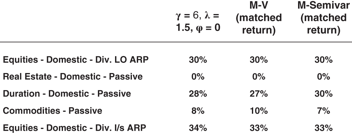
FIGURE 5.2 Comparison with Mean-Variance and Mean-Semivariance Frameworks When Returns Are Matched
To demonstrate formally our lack of dependence on higher moments for our current asset list (and underlying capital market assumptions), Figure 5.2 compares optimizer results for our three-dimensional utility function (![]() ,
, ![]() , and
, and ![]() ) to the mean-variance and mean-semivariance frameworks for a set return level. Mean-semivariance is just like M-V except it only considers volatility when it is to the downside (AKA semivariance), a simple system for accounting for the intuitive asymmetric preferences toward upside over downside, which we indeed fully capture via
) to the mean-variance and mean-semivariance frameworks for a set return level. Mean-semivariance is just like M-V except it only considers volatility when it is to the downside (AKA semivariance), a simple system for accounting for the intuitive asymmetric preferences toward upside over downside, which we indeed fully capture via ![]() in our prospect theory utility function. These two additional portfolios in Figure 5.2 have been optimized while holding constant the portfolio return to have the same expected return as our optimized three-dimensional utility portfolio. If our three-dimensional utility function indeed had outsized higher moment sensitivity compared to the two other target functions being optimized, then our three-dimensional utility optimization results would create distinct portfolios from these other methods due to those extra terms. In this case, however, we indeed see virtually equivalent portfolios in Figure 5.2 across the three methods, since our three-dimensional utility has negligible contributions from higher moment terms in this configuration. To be fair, we do see the mean-semivariance portfolio deviating from the mean-variance solution in Figure 5.2 by 3 percentage points; but the magnitude of this deviation is well within our allocation error bars, as reviewed in the last section of this chapter, so we do not flag that difference as very relevant.
in our prospect theory utility function. These two additional portfolios in Figure 5.2 have been optimized while holding constant the portfolio return to have the same expected return as our optimized three-dimensional utility portfolio. If our three-dimensional utility function indeed had outsized higher moment sensitivity compared to the two other target functions being optimized, then our three-dimensional utility optimization results would create distinct portfolios from these other methods due to those extra terms. In this case, however, we indeed see virtually equivalent portfolios in Figure 5.2 across the three methods, since our three-dimensional utility has negligible contributions from higher moment terms in this configuration. To be fair, we do see the mean-semivariance portfolio deviating from the mean-variance solution in Figure 5.2 by 3 percentage points; but the magnitude of this deviation is well within our allocation error bars, as reviewed in the last section of this chapter, so we do not flag that difference as very relevant.
With that said, our three-dimensional risk preference utility function is still an invaluable improvement from the traditional approach, as it provides for an insightful mapping of client preferences to portfolios based on real-world behaviors and allows for the systematic moderation of preferences based on client goals. Let's now take some time to refine our understanding of the value proposition of our three-dimensional utility function.
TO MPT OR NOT TO MPT?
Since higher moments have played a minimal role for our current asset configuration, an important question is: Can we pivot back to the MPT formulation? We obviously cannot if higher moments are relevant, which we really don't know unless we go through the full utility function optimization process in the first place. But for argument's sake, let's assume we know a priori that higher moments won't be critical—for instance, if we were always optimizing portfolios with our current five asset classes with the same joint return distribution.
Recall from Eq. (1.4) that the sensitivity of our utility function to the second moment is a function of the second derivative of our function, which is in fact a function of all three of our utility parameters ![]() ,
, ![]() , and
, and ![]() . In the current setting of marginal higher moment sensitivity, we can write our three-dimensional utility function as
. In the current setting of marginal higher moment sensitivity, we can write our three-dimensional utility function as
where r is the portfolio return and ![]() is a function of
is a function of ![]() ,
, ![]() , and
, and ![]() . For example, a utility function with very high loss aversion will certainly create strong aversion to volatility; and a utility function with reflection would push aversion to volatility in the opposite direction. Hopefully at this point it is rather intuitive to see how our two behavioral parameters affect
. For example, a utility function with very high loss aversion will certainly create strong aversion to volatility; and a utility function with reflection would push aversion to volatility in the opposite direction. Hopefully at this point it is rather intuitive to see how our two behavioral parameters affect ![]() . If it isn't clear, I encourage readers to review Figure 5.1 and the discussion in the previous section.
. If it isn't clear, I encourage readers to review Figure 5.1 and the discussion in the previous section.
As already noted, this reduction of the problem to a simple tradeoff between return and risk is on bright display in Figure 5.1. As one prefers less volatility, by virtue of preferring higher ![]() , higher
, higher ![]() , and no reflection
, and no reflection ![]() —which will all make
—which will all make ![]() go up—one clearly sees a shift to the last three assets, precisely those assets we labeled as “diversifying” in Chapter 3. The most extreme example of this would be the third column of the matrix at the bottom left of Figure 5.1 (
go up—one clearly sees a shift to the last three assets, precisely those assets we labeled as “diversifying” in Chapter 3. The most extreme example of this would be the third column of the matrix at the bottom left of Figure 5.1 (![]() ,
, ![]() , and
, and ![]() ) where we see the highest allocation to diversifying assets among all portfolios.
) where we see the highest allocation to diversifying assets among all portfolios.
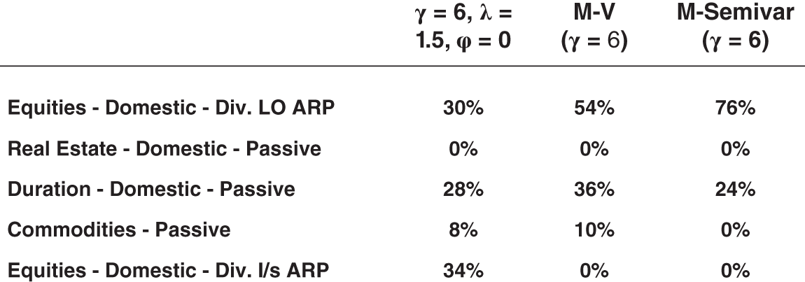
FIGURE 5.3 Comparison with Mean-Variance and Mean-Semivariance Frameworks
We could justify the need for our additional parameters if we assumed people did not have access to ![]() and could only ascertain
and could only ascertain ![]() . Figure 5.3 shows the recommended portfolio deploying three frameworks. The first is our three-dimensional utility function, with
. Figure 5.3 shows the recommended portfolio deploying three frameworks. The first is our three-dimensional utility function, with ![]() ,
, ![]() , and
, and ![]() , the second being mean-variance with
, the second being mean-variance with ![]() , and the third being mean-semivariance with
, and the third being mean-semivariance with ![]() . As you can see, while all these portfolios have
. As you can see, while all these portfolios have ![]() , they produce very different portfolios. Hence, a mistaken application of
, they produce very different portfolios. Hence, a mistaken application of ![]() in the place of
in the place of ![]() can lead to very misleading portfolios.2
can lead to very misleading portfolios.2
If we are careful though, we should be able to measure ![]() carefully, rather than
carefully, rather than ![]() , and we could avoid deploying the wrong optimization coefficient. But once we focus on measuring just
, and we could avoid deploying the wrong optimization coefficient. But once we focus on measuring just ![]() (instead of
(instead of ![]() ,
, ![]() , and
, and ![]() ), we lose an incredible amount of detail about our client that helps build intuition behind our process of building a portfolio for them. In my experience, this information is incredibly well received by the client, as they are generally interested in a more nuanced dissection of their personality rather than an effective representation. The three traits we are dissecting in our three-dimensional risk profile are part of the client's everyday life, and it is precisely that color that clients really appreciate a dialogue in. For instance, loss aversion relates to the type of phone case one buys, or it relates to how much life insurance one would be inclined to buy. It is this kind of information clients really enjoy seeing fleshed out as they gain a nuanced understanding of their own behavior. And it is wonderful to see how quickly the three risk preferences can help a client with daily decisions of all kinds outside the investment portfolio, with the proper education on the subject. In addition, this more detailed personality discovery process generally helps the client validate the advisor's process by demonstrating to them that the traits being diagnosed by the three-dimensional risk profile align with their actual behavior.3 Hence, the three-dimensional utility measurement process should provide an engaging process for clients with the welcome benefit of validating the advisor's process in the eye of the client.
), we lose an incredible amount of detail about our client that helps build intuition behind our process of building a portfolio for them. In my experience, this information is incredibly well received by the client, as they are generally interested in a more nuanced dissection of their personality rather than an effective representation. The three traits we are dissecting in our three-dimensional risk profile are part of the client's everyday life, and it is precisely that color that clients really appreciate a dialogue in. For instance, loss aversion relates to the type of phone case one buys, or it relates to how much life insurance one would be inclined to buy. It is this kind of information clients really enjoy seeing fleshed out as they gain a nuanced understanding of their own behavior. And it is wonderful to see how quickly the three risk preferences can help a client with daily decisions of all kinds outside the investment portfolio, with the proper education on the subject. In addition, this more detailed personality discovery process generally helps the client validate the advisor's process by demonstrating to them that the traits being diagnosed by the three-dimensional risk profile align with their actual behavior.3 Hence, the three-dimensional utility measurement process should provide an engaging process for clients with the welcome benefit of validating the advisor's process in the eye of the client.
But here comes the hammer: up to this point in our discussion of approximating our three-dimensional function with ![]() , we have assumed there are no financial goals to be accounted for. In Chapter 2, we introduced a system that moderated our three risk preferences independently based on our client's standard of living risk (SLR). In some configuration of the universe, which is not the one we live in, the three-dimensional parameters' moderation may have been collapsible into a system that is squarely focused on
, we have assumed there are no financial goals to be accounted for. In Chapter 2, we introduced a system that moderated our three risk preferences independently based on our client's standard of living risk (SLR). In some configuration of the universe, which is not the one we live in, the three-dimensional parameters' moderation may have been collapsible into a system that is squarely focused on ![]() . But because our goals-based moderations of the three parameters don't all go in the same direction of portfolio volatility, we can't do this. For example, when SLR is high, we are expected to moderate
. But because our goals-based moderations of the three parameters don't all go in the same direction of portfolio volatility, we can't do this. For example, when SLR is high, we are expected to moderate ![]() down and
down and ![]() up. But these two moderations push the portfolio in different directions regarding volatility. For example, starting from a portfolio with
up. But these two moderations push the portfolio in different directions regarding volatility. For example, starting from a portfolio with ![]() ,
, ![]() , and
, and ![]() in Figure 5.1, moderating just risk aversion up lowers portfolio volatility while moderating just loss aversion down increases portfolio volatility. It is thus impossible to properly moderate our three-dimensional risk preferences for financial goals with a single generalized risk aversion coefficient, because one of our two irrational preferences (loss aversion) is moderated toward a higher volatility portfolio, in the opposite direction of our other two parameters.
in Figure 5.1, moderating just risk aversion up lowers portfolio volatility while moderating just loss aversion down increases portfolio volatility. It is thus impossible to properly moderate our three-dimensional risk preferences for financial goals with a single generalized risk aversion coefficient, because one of our two irrational preferences (loss aversion) is moderated toward a higher volatility portfolio, in the opposite direction of our other two parameters.
ASSET ALLOCATION SENSITIVITY
A key criterion for our practical asset allocation framework was to build a system that wouldn't be highly sensitive to changes in the underlying capital market assumptions; otherwise we would require forecasting precision that is out of our reach. Figure 1.5 showcased just how sensitive a portfolio allocation could be with only minimal changes to return expectations if the assets are very similar—precisely the behavior we want to avoid. So, how do we measure this sensitivity without sitting here and constantly rerunning our optimizer with different assumptions to see how much the recommended portfolios change?
One succinct solution is to deploy the bootstrap method once again, a technique we are now very familiar with after Chapter 4. To recap: we created random samples of the full dataset to estimate the moment of interest and then repeated that process many times to create a distribution of the estimate itself, whose width we used as error bars to our estimate. Here, we are interested in the distribution of each asset's recommended asset allocation; so, we will create a random sample of the joint return distribution input as our optimizer's outcome forecasts, find the optimal portfolios, and then repeat this process many times to find a distribution of the recommended portfolio allocations, creating error bars around our recommended asset allocations.
Figure 5.4 shows the asset allocation results from Figure 5.1 for a single value of risk aversion ![]() , where we have now added our bootstrapped error bars on each asset's recommended allocation, where two striking features stand out. The first is that the error bars are not that small! This may surprise some readers, who have most likely never seen error bars on their asset allocations before; but the results may also be intuitive at this point after our results on moment estimation error from Chapter 4, where our error bars were not as small as we would have liked.
, where we have now added our bootstrapped error bars on each asset's recommended allocation, where two striking features stand out. The first is that the error bars are not that small! This may surprise some readers, who have most likely never seen error bars on their asset allocations before; but the results may also be intuitive at this point after our results on moment estimation error from Chapter 4, where our error bars were not as small as we would have liked.

FIGURE 5.4 Error Bars on Optimization Results for Selected  ,
,  , and
, and 
On this point I would say that, similar to the messaging from Chapter 4 on moment estimation error, in the world of noisy estimation of economically and behaviorally motivated risk premia with limited data, we are actually doing fine with these error bars. The larger takeaway is that we, as fiduciaries, should always be mindful of error bars in our research process. For example, running an optimizer based on very limited historical data would be irresponsible regarding estimation error. Additionally, we should be careful when we split hairs on our client profile buckets. For instance, if you bucket your clients into 100 distinct levels of risk aversion, I would immediately challenge whether your estimation error allows you to distinguish portfolios with that level of accuracy.
The second main takeaway from Figure 5.4 is that the error bars go down as our generalized risk aversion goes up. This makes a lot of sense, since the error bars in the riskier portfolios are predominantly driven by the estimation error associated with the riskier assets, which by their very nature have higher estimation error due to their higher volatility.
In Chapter 3 we saw that, on a percentage basis, the error bars on volatility were much smaller than the error bars on returns. This result is a primary reason why risk parity strategies have gained in popularity.4 But just how compelling is the decrease in error bars that risk parity offers? Figure 5.5 shows the risk parity portfolio with error bars, alongside a utility-maximized portfolio with similar amounts of total equity plus real estate allocation (which is a quick way to normalize away the effects of volatility on error bars reviewed in the previous paragraph). As you can see, the risk parity error bars are a fraction of the size of the error bars on a portfolio with similar levels of risk that was built from our utility maximization process. While the error bars in risk parity are indeed eye-popping, the major issue with this routine is that it is completely agnostic of client specifics, appropriate only for clients with high generalized risk aversion (as evidenced from the allocations matching a utility-optimal portfolio with loss aversion of 2), and in the environment where third and higher moments are inconsequential. Nonetheless, risk parity is an interesting case study to help us build our intuition around error bars.

FIGURE 5.5 Error Bars on Utility Optimization vs. Risk Parity
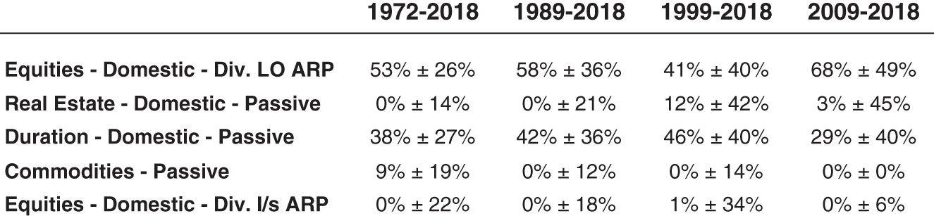
FIGURE 5.6 Error Bars on Optimization Results as a Function of Sample Size ( ,
,  , and
, and  )
)
Figure 5.6 shows the optimization results for a portfolio with ![]() ,
, ![]() , and
, and ![]() as we change the lookback history used for our outcome forecasts. As you can see, as sample size is increased, the error bars on our dominant allocations decrease, exactly the behavior we would hope for. What we are seeing is estimation error going down as the sample size increases, which is directly leading to smaller error bars on our prescribed portfolios.
as we change the lookback history used for our outcome forecasts. As you can see, as sample size is increased, the error bars on our dominant allocations decrease, exactly the behavior we would hope for. What we are seeing is estimation error going down as the sample size increases, which is directly leading to smaller error bars on our prescribed portfolios.
Finally, Figure 5.7 explores asset allocation sensitivity due to asset redundancy by comparing our results with those of portfolios that include redundant assets. The analysis begins with the ![]() ,
, ![]() , and
, and ![]() portfolio with the five assets we have focused on throughout the chapter; we then proceed to add US small caps to the portfolio to analyze the effect of adding an asset significantly redundant to our core equity holding. Next, we add the 10-year Treasury asset to create a similar effect relative to our core longer duration asset. Finally, we see the bootstrapped results for a portfolio that includes both redundant assets.5
portfolio with the five assets we have focused on throughout the chapter; we then proceed to add US small caps to the portfolio to analyze the effect of adding an asset significantly redundant to our core equity holding. Next, we add the 10-year Treasury asset to create a similar effect relative to our core longer duration asset. Finally, we see the bootstrapped results for a portfolio that includes both redundant assets.5
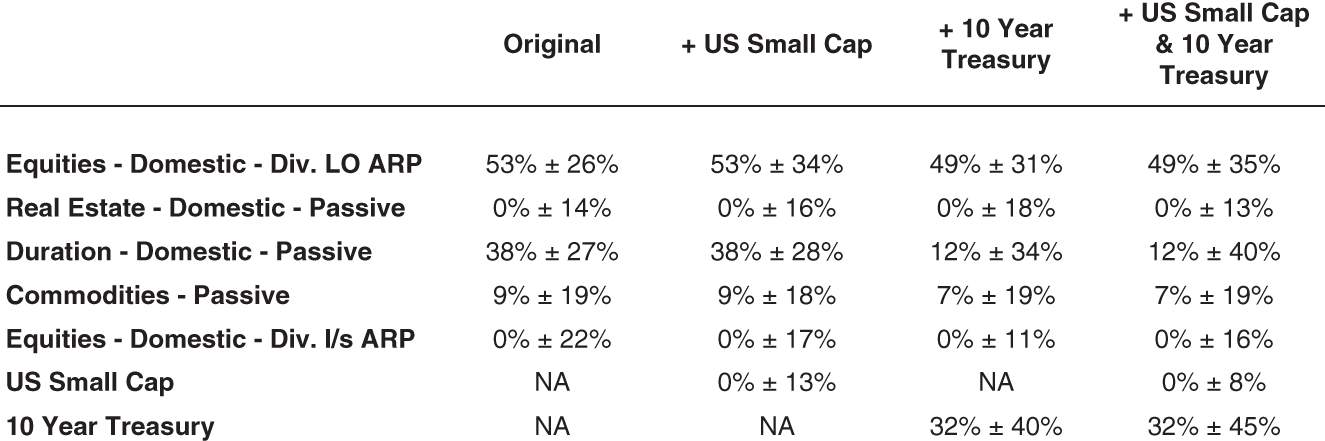
FIGURE 5.7 Error Bars on Optimization Results as a Function of Asset Universe ( ,
,  , and
, and  )
)
In the case of adding just US small caps, we see some increase in error bars for our core equity holding, but nothing crazy. Notice, however, that this new holding we have added also is not pulling any assets away from our core allocation. So, despite our intuitive sense that US small caps would be redundant enough to compete with our core US equity asset, the optimizer is not flagging it as a compelling relative asset, helping keep the error bars low. The 10-year Treasury asset, on the other hand, introduces significantly more error into the mix due to its redundant nature relative to our longer duration asset, which is clearly being flagged by the optimizer as more interesting relative to our core duration asset. And these were just two assets picked out of a hat; if one were to create a portfolio with 30 assets, many of which were similar, we would see much more error bar chaos prevail.
FINAL REMARKS
This book has brought modern features from behavioral economics into our client's risk profile, along with a modernized system for incorporating financial goals into the asset allocation process, and has enabled incorporation of more realistic higher moment behavior into the asset allocation process. This book has also focused on creating a practical framework by enabling streamlined forecasting from history while tackling the challenges that estimation error presents by deploying statistically sound estimation techniques and avoiding redundant assets.
The goal of this book was to empower financial advisors to confidently build portfolios that are truly personalized for their clients. I hope we have indeed taken a solid step toward such a modern yet practical asset allocation framework.
NOTES
- 1 Treasuries are represented by constant maturity indices from the Center for Research in Security Prices at the University of Chicago's Booth School of Business (CRSP®); equity data is from Ken French's online library with all factor assets following conventional definitions; real estate is represented by the FTSE Nareit US Real Estate Index; and commodities are expressed via the S&P GSCI Commodity Index.
- 2 We see an even more extreme discrepancy between our 3D utility and mean-semivariance because the risk metric of semivariance is a significantly smaller quantity than the volatility by definition, hence putting less weight on the risk side of the ledger for the optimizer, since it roughly only measures half the distribution width.
- 3 This client validation process is also one way the author has gained comfort with the questionnaires being deployed in Chapter 2, outside the more formal domain of psychometric testing of validity.
- 4 Risk parity allocations force each asset class to contribute the same amount of volatility to the portfolio.
- 5 The 10-year Treasury is represented by a constant maturity index from the Center for Research in Security Prices at the University of Chicago's Booth School of Business (CRSP®). US small cap data is from Ken French's online library, where we use the bottom quintile of equities sorted on size.
..................Content has been hidden....................
You can't read the all page of ebook, please click here login for view all page.